Example Algorithms
This section documents a number of example algorithms to complement the beginner tutorial, and show how other trading algorithms can be implemented using Catalyst.
Overview
- Buy BTC Simple: The simplest algorithm that introduces
the
initialize()andhandle_data()functions, and is used in the beginner tutorial to show how to run catalyst for the first time. - Buy and Hodl: A very straightforward buy and hold that
makes one single buy at the very beginning. Introduces the notions of
cash, management of outstandingorders, andorder_target_valueto place orders. It also introduces theanalyze()function to visualize the performance of our strategy using the external librarymatplotlib. - Dual Moving Average Crossover: A classic momentum
strategy used in the second part of the
beginner tutorial to introduce the
data.history()function. It makes a heavy use ofmatplotliblibrary in theanalyze()function to chart the performance of the algorithm. - Mean Reversion Algorithm: Another simple momentum strategy that is used in our two-part video tutorial to show how to get started in backtesting and live trading with Catalyst.
- Simple Universe: This code provides the ‘universe’ of available trading pairs on a given exchange on any given day. You can use this code to dynamically select which currency pairs you want to trade each day of your strategy. This example does not make any trades.
- Portfolio Optimization: Use this code to execute a portfolio optimization model. This strategy will select the portfolio with the maximum Sharpe Ratio. The parameters are set to use 180 days of historical data and rebalance every 30 days. This code was used in writting the following article: Markowitz Portfolio Optimization for Cryptocurrencies.
Buy BTC Simple Algorithm
Source code: examples/buy_btc_simple.py
'''
  Run this example, by executing the following from your terminal:
    catalyst ingest-exchange -x bitfinex -f daily -i btc_usdt
    catalyst run -f buy_btc_simple.py -x bitfinex --start 2016-1-1 --end 2017-9-30 -o buy_btc_simple_out.pickle

  If you want to run this code using another exchange, make sure that
  the asset is available on that exchange. For example, if you were to run
  it for exchange Poloniex, you would need to edit the following line:

    context.asset = symbol('btc_usdt')     # note 'usdt' instead of 'usd'

  and specify exchange poloniex as follows:
  catalyst ingest-exchange -x poloniex -f daily -i btc_usdt
  catalyst run -f buy_btc_simple.py -x poloniex --start 2016-1-1 --end 2017-9-30 -o buy_btc_simple_out.pickle

  To see which assets are available on each exchange, visit:
  https://www.enigma.co/catalyst/status
'''

from catalyst.api import order, record, symbol

def initialize(context):
    context.asset = symbol('btc_usd')

def handle_data(context, data):
    order(context.asset, 1)
    record(btc = data.current(context.asset, 'price'))
This simple algorithm does not produce any output nor displays any chart.
Buy and Hodl Algorithm
Source code: examples/buy_and_hodl.py
First ingest the historical pricing data needed to run this algorithm:
catalyst ingest-exchange -x bitfinex -f daily -i btc_usd
Then, you can run the code below with the following command:
catalyst run -f buy_and_hodl.py --start 2015-3-1 --end 2017-10-31 --capital-base 100000 -x bitfinex -c btc -o bah.pickle
or using the same parameters specified in the run_algorithm() function at the end of the file:
python buy_and_hodl.py
This command will run the trading algorithm in the specified time range and
plot the resulting performance using the matplotlib library. You can choose any
date interval with the --start and --end parameters, but bear in mind
that 2015-3-1 is the earliest date that Catalyst supports (if you choose an
earlier date, you’ll get an error), and the most recent date you can choose is
one day prior to the current date.
#!/usr/bin/env python
#
# Copyright 2017 Enigma MPC, Inc.
# Copyright 2015 Quantopian, Inc.
#
# Licensed under the Apache License, Version 2.0 (the "License");
# you may not use this file except in compliance with the License.
# You may obtain a copy of the License at
#
#     http://www.apache.org/licenses/LICENSE-2.0
#
# Unless required by applicable law or agreed to in writing, software
# distributed under the License is distributed on an "AS IS" BASIS,
# WITHOUT WARRANTIES OR CONDITIONS OF ANY KIND, either express or implied.
# See the License for the specific language governing permissions and
# limitations under the License.
import pandas as pd
import matplotlib.pyplot as plt

from catalyst import run_algorithm
from catalyst.api import (order_target_value, symbol, record,
    cancel_order, get_open_orders, )


def initialize(context):
    context.ASSET_NAME = 'btc_usd'
    context.TARGET_HODL_RATIO = 0.8
    context.RESERVE_RATIO = 1.0 - context.TARGET_HODL_RATIO

    context.is_buying = True
    context.asset = symbol(context.ASSET_NAME)

    context.i = 0


def handle_data(context, data):
    context.i += 1

    starting_cash = context.portfolio.starting_cash
    target_hodl_value = context.TARGET_HODL_RATIO * starting_cash
    reserve_value = context.RESERVE_RATIO * starting_cash

    # Cancel any outstanding orders
    orders = get_open_orders(context.asset) or []
    for order in orders:
        cancel_order(order)

    # Stop buying after passing the reserve threshold
    cash = context.portfolio.cash
    if cash <= reserve_value:
        context.is_buying = False

    # Retrieve current asset price from pricing data
    price = data.current(context.asset, 'price')

    # Check if still buying and could (approximately) afford another purchase
    if context.is_buying and cash > price:
        print('buying')
        # Place order to make position in asset equal to target_hodl_value
        order_target_value(
            context.asset,
            target_hodl_value,
            limit_price=price * 1.1,
        )

    record(
        price=price,
        volume=data.current(context.asset, 'volume'),
        cash=cash,
        starting_cash=context.portfolio.starting_cash,
        leverage=context.account.leverage,
    )


def analyze(context=None, results=None):

    # Plot the portfolio and asset data.
    ax1 = plt.subplot(611)
    results[['portfolio_value']].plot(ax=ax1)
    ax1.set_ylabel('Portfolio Value (USD)')

    ax2 = plt.subplot(612, sharex=ax1)
    ax2.set_ylabel('{asset} (USD)'.format(asset=context.ASSET_NAME))
    results[['price']].plot(ax=ax2)

    trans = results.ix[[t != [] for t in results.transactions]]
    buys = trans.ix[
        [t[0]['amount'] > 0 for t in trans.transactions]
    ]
    ax2.scatter(
        buys.index.to_pydatetime(),
        results.price[buys.index],
        marker='^',
        s=100,
        c='g',
        label=''
    )

    ax3 = plt.subplot(613, sharex=ax1)
    results[['leverage', 'alpha', 'beta']].plot(ax=ax3)
    ax3.set_ylabel('Leverage ')

    ax4 = plt.subplot(614, sharex=ax1)
    results[['starting_cash', 'cash']].plot(ax=ax4)
    ax4.set_ylabel('Cash (USD)')

    results[[
        'treasury',
        'algorithm',
        'benchmark',
    ]] = results[[
        'treasury_period_return',
        'algorithm_period_return',
        'benchmark_period_return',
    ]]

    ax5 = plt.subplot(615, sharex=ax1)
    results[[
        'treasury',
        'algorithm',
        'benchmark',
    ]].plot(ax=ax5)
    ax5.set_ylabel('Percent Change')

    ax6 = plt.subplot(616, sharex=ax1)
    results[['volume']].plot(ax=ax6)
    ax6.set_ylabel('Volume (mCoins/5min)')

    plt.legend(loc=3)

    # Show the plot.
    plt.gcf().set_size_inches(18, 8)
    plt.show()


if __name__ == '__main__':
    run_algorithm(
        capital_base=10000,
        data_frequency='daily',
        initialize=initialize,
        handle_data=handle_data,
        analyze=analyze,
        exchange_name='bitfinex',
        algo_namespace='buy_and_hodl',
        base_currency='usd',
        start=pd.to_datetime('2015-03-01', utc=True),
        end=pd.to_datetime('2017-10-31', utc=True),
    )

Dual Moving Average Crossover
Source Code: examples/dual_moving_average.py
This strategy is covered in detail in the last part of this tutorial.
import numpy as np
import pandas as pd
from logbook import Logger
import matplotlib.pyplot as plt

from catalyst import run_algorithm
from catalyst.api import (order, record, symbol, order_target_percent,
        get_open_orders)
from catalyst.exchange.stats_utils import extract_transactions

NAMESPACE = 'dual_moving_average'
log = Logger(NAMESPACE)

def initialize(context):
    context.i = 0
    context.asset = symbol('ltc_usd')
    context.base_price = None


def handle_data(context, data):
    # define the windows for the moving averages
    short_window = 50
    long_window = 200

    # Skip as many bars as long_window to properly compute the average
    context.i += 1
    if context.i < long_window:
       return

    # Compute moving averages calling data.history() for each
    # moving average with the appropriate parameters. We choose to use
    # minute bars for this simulation -> freq="1m"
    # Returns a pandas dataframe.
    short_mavg = data.history(context.asset, 'price',
                        bar_count=short_window, frequency="1m").mean()
    long_mavg = data.history(context.asset, 'price',
                        bar_count=long_window, frequency="1m").mean()

    # Let's keep the price of our asset in a more handy variable
    price = data.current(context.asset, 'price')

    # If base_price is not set, we use the current value. This is the
    # price at the first bar which we reference to calculate price_change.
    if context.base_price is None:
        context.base_price = price
    price_change = (price - context.base_price) / context.base_price

    # Save values for later inspection
    record(price=price,
           cash=context.portfolio.cash,
           price_change=price_change,
           short_mavg=short_mavg,
           long_mavg=long_mavg)

    # Since we are using limit orders, some orders may not execute immediately
    # we wait until all orders are executed before considering more trades.
    orders = get_open_orders(context.asset)
    if len(orders) > 0:
        return

    # Exit if we cannot trade
    if not data.can_trade(context.asset):
        return

    # We check what's our position on our portfolio and trade accordingly
    pos_amount = context.portfolio.positions[context.asset].amount

    # Trading logic
    if short_mavg > long_mavg and pos_amount == 0:
       # we buy 100% of our portfolio for this asset
       order_target_percent(context.asset, 1)
    elif short_mavg < long_mavg and pos_amount > 0:
       # we sell all our positions for this asset
       order_target_percent(context.asset, 0)


def analyze(context, perf):

    # Get the base_currency that was passed as a parameter to the simulation
    base_currency = context.exchanges.values()[0].base_currency.upper()

    # First chart: Plot portfolio value using base_currency
    ax1 = plt.subplot(411)
    perf.loc[:, ['portfolio_value']].plot(ax=ax1)
    ax1.legend_.remove()
    ax1.set_ylabel('Portfolio Value\n({})'.format(base_currency))
    start, end = ax1.get_ylim()
    ax1.yaxis.set_ticks(np.arange(start, end, (end-start)/5))

    # Second chart: Plot asset price, moving averages and buys/sells
    ax2 = plt.subplot(412, sharex=ax1)
    perf.loc[:, ['price','short_mavg','long_mavg']].plot(ax=ax2, label='Price')
    ax2.legend_.remove()
    ax2.set_ylabel('{asset}\n({base})'.format(
        asset = context.asset.symbol,
        base = base_currency
        ))
    start, end = ax2.get_ylim()
    ax2.yaxis.set_ticks(np.arange(start, end, (end-start)/5))

    transaction_df = extract_transactions(perf)
    if not transaction_df.empty:
        buy_df = transaction_df[transaction_df['amount'] > 0]
        sell_df = transaction_df[transaction_df['amount'] < 0]
        ax2.scatter(
            buy_df.index.to_pydatetime(),
            perf.loc[buy_df.index, 'price'],
            marker='^',
            s=100,
            c='green',
            label=''
        )
        ax2.scatter(
            sell_df.index.to_pydatetime(),
            perf.loc[sell_df.index, 'price'],
            marker='v',
            s=100,
            c='red',
            label=''
        )

    # Third chart: Compare percentage change between our portfolio
    # and the price of the asset
    ax3 = plt.subplot(413, sharex=ax1)
    perf.loc[:, ['algorithm_period_return', 'price_change']].plot(ax=ax3)
    ax3.legend_.remove()
    ax3.set_ylabel('Percent Change')
    start, end = ax3.get_ylim()
    ax3.yaxis.set_ticks(np.arange(start, end, (end-start)/5))

    # Fourth chart: Plot our cash
    ax4 = plt.subplot(414, sharex=ax1)
    perf.cash.plot(ax=ax4)
    ax4.set_ylabel('Cash\n({})'.format(base_currency))
    start, end = ax4.get_ylim()
    ax4.yaxis.set_ticks(np.arange(0, end, end/5))

    plt.show()


if __name__ == '__main__':
    run_algorithm(
            capital_base=1000,
            data_frequency='minute',
            initialize=initialize,
            handle_data=handle_data,
            analyze=analyze,
            exchange_name='bitfinex',
            algo_namespace=NAMESPACE,
            base_currency='usd',
            start=pd.to_datetime('2017-9-22', utc=True),
            end=pd.to_datetime('2017-9-23', utc=True),
        )

Mean Reversion Algorithm
Source code: examples/mean_reversion_simple.py
This algorithm is based on a simple momentum strategy. When the cryptoasset goes up quickly, we’re going to buy; when it goes down quickly, we’re going to sell. Hopefully, we’ll ride the waves.
We are choosing to backtest this trading algorithm with the neo_usd currency
pairon the Bitfinex exchange. Thus, first ingest the historical pricing data
that we need, with minute resolution:
catalyst ingest-exchange -x bitfinex -f minute -i neo_usd
To run this algorithm, we are opting for the Python interpreter, instead of the command line (CLI). All of the parameters for the simulation are specified in lines 218-245, so in order to run the algorithm we just type:
python mean_reversion_simple.py
import os
import tempfile
import time

import numpy as np
import pandas as pd
import talib
from logbook import Logger

from catalyst import run_algorithm
from catalyst.api import symbol, record, order_target_percent, get_open_orders
from catalyst.exchange.stats_utils import extract_transactions
# We give a name to the algorithm which Catalyst will use to persist its state.
# In this example, Catalyst will create the `.catalyst/data/live_algos`
# directory. If we stop and start the algorithm, Catalyst will resume its
# state using the files included in the folder.
from catalyst.utils.paths import ensure_directory

NAMESPACE = 'mean_reversion_simple'
log = Logger(NAMESPACE)


# To run an algorithm in Catalyst, you need two functions: initialize and
# handle_data.

def initialize(context):
    # This initialize function sets any data or variables that you'll use in
    # your algorithm.  For instance, you'll want to define the trading pair (or
    # trading pairs) you want to backtest.  You'll also want to define any
    # parameters or values you're going to use.

    # In our example, we're looking at Neo in USD.
    context.neo_eth = symbol('neo_usd')
    context.base_price = None
    context.current_day = None

    context.RSI_OVERSOLD = 30
    context.RSI_OVERBOUGHT = 80
    context.CANDLE_SIZE = '15T'

    context.start_time = time.time()


def handle_data(context, data):
    # This handle_data function is where the real work is done.  Our data is
    # minute-level tick data, and each minute is called a frame.  This function
    # runs on each frame of the data.

    # We flag the first period of each day.
    # Since cryptocurrencies trade 24/7 the `before_trading_starts` handle
    # would only execute once. This method works with minute and daily
    # frequencies.
    today = data.current_dt.floor('1D')
    if today != context.current_day:
        context.traded_today = False
        context.current_day = today

    # We're computing the volume-weighted-average-price of the security
    # defined above, in the context.neo_eth variable.  For this example, we're
    # using three bars on the 15 min bars.

    # The frequency attribute determine the bar size. We use this convention
    # for the frequency alias:
    # http://pandas.pydata.org/pandas-docs/stable/timeseries.html#offset-aliases
    prices = data.history(
        context.neo_eth,
        fields='close',
        bar_count=50,
        frequency=context.CANDLE_SIZE
    )

    # Ta-lib calculates various technical indicator based on price and
    # volume arrays.

    # In this example, we are comp
    rsi = talib.RSI(prices.values, timeperiod=14)

    # We need a variable for the current price of the security to compare to
    # the average. Since we are requesting two fields, data.current()
    # returns a DataFrame with
    current = data.current(context.neo_eth, fields=['close', 'volume'])
    price = current['close']

    # If base_price is not set, we use the current value. This is the
    # price at the first bar which we reference to calculate price_change.
    if context.base_price is None:
        context.base_price = price

    price_change = (price - context.base_price) / context.base_price
    cash = context.portfolio.cash

    # Now that we've collected all current data for this frame, we use
    # the record() method to save it. This data will be available as
    # a parameter of the analyze() function for further analysis.
    record(
        price=price,
        volume=current['volume'],
        price_change=price_change,
        rsi=rsi[-1],
        cash=cash
    )

    # We are trying to avoid over-trading by limiting our trades to
    # one per day.
    if context.traded_today:
        return

    # Since we are using limit orders, some orders may not execute immediately
    # we wait until all orders are executed before considering more trades.
    orders = get_open_orders(context.neo_eth)
    if len(orders) > 0:
        return

    # Exit if we cannot trade
    if not data.can_trade(context.neo_eth):
        return

    # Another powerful built-in feature of the Catalyst backtester is the
    # portfolio object.  The portfolio object tracks your positions, cash,
    # cost basis of specific holdings, and more.  In this line, we calculate
    # how long or short our position is at this minute.
    pos_amount = context.portfolio.positions[context.neo_eth].amount

    if rsi[-1] <= context.RSI_OVERSOLD and pos_amount == 0:
        log.info(
            '{}: buying - price: {}, rsi: {}'.format(
                data.current_dt, price, rsi[-1]
            )
        )
        # Set a style for limit orders,
        limit_price = price * 1.005
        order_target_percent(
            context.neo_eth, 1, limit_price=limit_price
        )
        context.traded_today = True

    elif rsi[-1] >= context.RSI_OVERBOUGHT and pos_amount > 0:
        log.info(
            '{}: selling - price: {}, rsi: {}'.format(
                data.current_dt, price, rsi[-1]
            )
        )
        limit_price = price * 0.995
        order_target_percent(
            context.neo_eth, 0, limit_price=limit_price
        )
        context.traded_today = True


def analyze(context=None, perf=None):
    end = time.time()
    log.info('elapsed time: {}'.format(end - context.start_time))

    import matplotlib.pyplot as plt
    # The base currency of the algo exchange
    base_currency = context.exchanges.values()[0].base_currency.upper()

    # Plot the portfolio value over time.
    ax1 = plt.subplot(611)
    perf.loc[:, 'portfolio_value'].plot(ax=ax1)
    ax1.set_ylabel('Portfolio\nValue\n({})'.format(base_currency))

    # Plot the price increase or decrease over time.
    ax2 = plt.subplot(612, sharex=ax1)
    perf.loc[:, 'price'].plot(ax=ax2, label='Price')

    ax2.set_ylabel('{asset}\n({base})'.format(
        asset=context.neo_eth.symbol, base=base_currency
    ))

    transaction_df = extract_transactions(perf)
    if not transaction_df.empty:
        buy_df = transaction_df[transaction_df['amount'] > 0]
        sell_df = transaction_df[transaction_df['amount'] < 0]
        ax2.scatter(
            buy_df.index.to_pydatetime(),
            perf.loc[buy_df.index.floor('1 min'), 'price'],
            marker='^',
            s=100,
            c='green',
            label=''
        )
        ax2.scatter(
            sell_df.index.to_pydatetime(),
            perf.loc[sell_df.index.floor('1 min'), 'price'],
            marker='v',
            s=100,
            c='red',
            label=''
        )

    ax4 = plt.subplot(613, sharex=ax1)
    perf.loc[:, 'cash'].plot(
        ax=ax4, label='Base Currency ({})'.format(base_currency)
    )
    ax4.set_ylabel('Cash\n({})'.format(base_currency))

    perf['algorithm'] = perf.loc[:, 'algorithm_period_return']

    ax5 = plt.subplot(614, sharex=ax1)
    perf.loc[:, ['algorithm', 'price_change']].plot(ax=ax5)
    ax5.set_ylabel('Percent\nChange')

    ax6 = plt.subplot(615, sharex=ax1)
    perf.loc[:, 'rsi'].plot(ax=ax6, label='RSI')
    ax6.set_ylabel('RSI')
    ax6.axhline(context.RSI_OVERBOUGHT, color='darkgoldenrod')
    ax6.axhline(context.RSI_OVERSOLD, color='darkgoldenrod')

    if not transaction_df.empty:
        ax6.scatter(
            buy_df.index.to_pydatetime(),
            perf.loc[buy_df.index.floor('1 min'), 'rsi'],
            marker='^',
            s=100,
            c='green',
            label=''
        )
        ax6.scatter(
            sell_df.index.to_pydatetime(),
            perf.loc[sell_df.index.floor('1 min'), 'rsi'],
            marker='v',
            s=100,
            c='red',
            label=''
        )
    plt.legend(loc=3)
    start, end = ax6.get_ylim()
    ax6.yaxis.set_ticks(np.arange(0, end, end/5))

    # Show the plot.
    plt.gcf().set_size_inches(18, 8)
    plt.show()
    pass


if __name__ == '__main__':
    # The execution mode: backtest or live
    MODE = 'backtest'

    if MODE == 'backtest':
        folder = os.path.join(
            tempfile.gettempdir(), 'catalyst', NAMESPACE
        )
        ensure_directory(folder)

        timestr = time.strftime('%Y%m%d-%H%M%S')
        out = os.path.join(folder, '{}.p'.format(timestr))
        # catalyst run -f catalyst/examples/mean_reversion_simple.py -x bitfinex -s 2017-10-1 -e 2017-11-10 -c usdt -n mean-reversion --data-frequency minute --capital-base 10000
        run_algorithm(
            capital_base=10000,
            data_frequency='minute',
            initialize=initialize,
            handle_data=handle_data,
            analyze=analyze,
            exchange_name='bitfinex',
            algo_namespace=NAMESPACE,
            base_currency='usd',
            start=pd.to_datetime('2017-10-01', utc=True),
            end=pd.to_datetime('2017-11-10', utc=True),
            output=out
        )
        log.info('saved perf stats: {}'.format(out))

    elif MODE == 'live':
        run_algorithm(
            capital_base=0.5,
            initialize=initialize,
            handle_data=handle_data,
            analyze=analyze,
            exchange_name='bittrex',
            live=True,
            algo_namespace=NAMESPACE,
            base_currency='usd',
            live_graph=False
        )

Notice the difference in performance between the charts above and those seen on this video tutorial at minute 8:10. The buy and sell orders are triggered at the same exact times, but the differences result from a more realistic slippage model implemented after the video was recorded, which executes the orders at slighlty different prices, but resulting in significant changes in performance of our strategy.
Simple Universe
Source code: examples/simple_universe.py
This example aims to provide an easy way for users to learn how to collect data from any given exchange and select a subset of the available currency pairs for trading. You simply need to specify the exchange and the market (base_currency) that you want to focus on. You will then see how to create a universe of assets, and filter it based the market you desire.
The example prints out the closing price of all the pairs for a given market in a given exchange every 30 minutes. The example also contains the OHLCV data with minute-resolution for the past seven days which could be used to create indicators. Use this code as the backbone to create your own trading strategy.
The lookback_date variable is used to ensure data for a coin existed on the lookback period specified.
To run, execute the following two commands in a terminal (inside catalyst environment). The first one retrieves all the pricing data needed for this script to run (only needs to be run once), and the second one executes this script with the parameters specified in the run_algorithm() call at the end of the file:
catalyst ingest-exchange -x bitfinex -f minute
python simple_universe.py
Credits: This code was originally submitted by Abner Ayala-Acevedo. Thank you!
from datetime import timedelta

import numpy as np
import pandas as pd

from catalyst import run_algorithm
from catalyst.exchange.utils.exchange_utils import get_exchange_symbols
from catalyst.api import (symbols, )


def initialize(context):
    context.i = -1  # minute counter
    context.exchange = context.exchanges.values()[0].name.lower()
    context.base_currency = context.exchanges.values()[0].base_currency.lower()


def handle_data(context, data):
    context.i += 1
    lookback_days = 7  # 7 days

    # current date & time in each iteration formatted into a string
    now = data.current_dt
    date, time = now.strftime('%Y-%m-%d %H:%M:%S').split(' ')
    lookback_date = now - timedelta(days=lookback_days)
    # keep only the date as a string, discard the time
    lookback_date = lookback_date.strftime('%Y-%m-%d %H:%M:%S').split(' ')[0]

    one_day_in_minutes = 1440  # 60 * 24 assumes data_frequency='minute'
    # update universe everyday at midnight
    if not context.i % one_day_in_minutes:
        context.universe = universe(context, lookback_date, date)

    # get data every 30 minutes
    minutes = 30
    # get lookback_days of history data: that is 'lookback' number of bins
    lookback = one_day_in_minutes / minutes * lookback_days
    if not context.i % minutes and context.universe:
        # we iterate for every pair in the current universe
        for coin in context.coins:
            pair = str(coin.symbol)

            # Get 30 minute interval OHLCV data. This is the standard data
            # required for candlestick or indicators/signals. Return Pandas
            # DataFrames. 30T means 30-minute re-sampling of one minute data.
            # Adjust it to your desired time interval as needed.
            opened = fill(data.history(coin, 'open',
                                  bar_count=lookback, frequency='30T')).values
            high = fill(data.history(coin, 'high',
                                  bar_count=lookback, frequency='30T')).values
            low = fill(data.history(coin, 'low',
                                  bar_count=lookback, frequency='30T')).values
            close = fill(data.history(coin, 'price',
                                  bar_count=lookback, frequency='30T')).values
            volume = fill(data.history(coin, 'volume',
                                  bar_count=lookback, frequency='30T')).values

            # close[-1] is the last value in the set, which is the equivalent
            # to current price (as in the most recent value)
            # displays the minute price for each pair every 30 minutes
            print('{now}: {pair} -\tO:{o},\tH:{h},\tL:{c},\tC{c},\tV:{v}'.format(
                    now=now,
                    pair=pair,
                    o=opened[-1],
                    h=high[-1],
                    l=low[-1],
                    c=close[-1],
                    v=volume[-1],
                 ))

            # -------------------------------------------------------------
            # --------------- Insert Your Strategy Here -------------------
            # -------------------------------------------------------------


def analyze(context=None, results=None):
    pass


# Get the universe for a given exchange and a given base_currency market
# Example: Poloniex BTC Market
def universe(context, lookback_date, current_date):
    # get all the pairs for the given exchange
    json_symbols = get_exchange_symbols(context.exchange)
    # convert into a DataFrame for easier processing
    df = pd.DataFrame.from_dict(json_symbols).transpose().astype(str)
    df['base_currency'] = df.apply(lambda row: row.symbol.split('_')[1],axis=1)
    df['market_currency'] = df.apply(lambda row: row.symbol.split('_')[0],axis=1)

    # Filter all the pairs to get only the ones for a given base_currency
    df = df[df['base_currency'] == context.base_currency]

    # Filter all the pairs to ensure that pair existed in the current date range
    df = df[df.start_date < lookback_date]
    df = df[df.end_daily >= current_date]
    context.coins = symbols(*df.symbol)  # convert all the pairs to symbols

    return df.symbol.tolist()


# Replace all NA, NAN or infinite values with its nearest value
def fill(series):
    if isinstance(series, pd.Series):
        return series.replace([np.inf, -np.inf], np.nan).ffill().bfill()
    elif isinstance(series, np.ndarray):
        return pd.Series(series).replace(
                     [np.inf, -np.inf], np.nan
                    ).ffill().bfill().values
    else:
        return series


if __name__ == '__main__':
    start_date = pd.to_datetime('2017-11-10', utc=True)
    end_date = pd.to_datetime('2017-11-13', utc=True)

    performance = run_algorithm(start=start_date, end=end_date,
                                capital_base=100.0,  # amount of base_currency
                                initialize=initialize,
                                handle_data=handle_data,
                                analyze=analyze,
                                exchange_name='bitfinex',
                                data_frequency='minute',
                                base_currency='btc',
                                live=False,
                                live_graph=False,
                                algo_namespace='simple_universe')
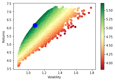
Portfolio Optimization
Use this code to execute a portfolio optimization model. This strategy will select the portfolio with the maximum Sharpe Ratio. The parameters are set to use 180 days of historical data and rebalance every 30 days. This code was used in writting the following article: Markowitz Portfolio Optimization for Cryptocurrencies.
'''
   You can run this code using the Python interpreter:

   $ python portfolio_optimization.py
'''

from __future__ import division
import os
import pytz
import numpy as np
import pandas as pd
from scipy.optimize import minimize
import matplotlib.pyplot as plt
from datetime import datetime

from catalyst.api import record, symbol, symbols, order_target_percent
from catalyst.utils.run_algo import run_algorithm

np.set_printoptions(threshold='nan', suppress=True)


def initialize(context):
   # Portfolio assets list
   context.assets = symbols('btc_usdt', 'eth_usdt', 'ltc_usdt', 'dash_usdt',
                            'xmr_usdt')
   context.nassets = len(context.assets)
   # Set the time window that will be used to compute expected return
   # and asset correlations
   context.window = 180
   # Set the number of days between each portfolio rebalancing
   context.rebalance_period = 30
   context.i = 0


def handle_data(context, data):
   # Only rebalance at the beggining of the algorithm execution and
   # every multiple of the rebalance period
   if context.i == 0 or context.i%context.rebalance_period == 0:
       n = context.window
       prices = data.history(context.assets, fields='price',
                             bar_count=n+1, frequency='1d')
       pr = np.asmatrix(prices)
       t_prices = prices.iloc[1:n+1]
       t_val = t_prices.values
       tminus_prices = prices.iloc[0:n]
       tminus_val = tminus_prices.values
       # Compute daily returns (r)
       r = np.asmatrix(t_val/tminus_val-1)
       # Compute the expected returns of each asset with the average
       # daily return for the selected time window
       m = np.asmatrix(np.mean(r, axis=0))
       # ###
       stds = np.std(r, axis=0)
       # Compute excess returns matrix (xr)
       xr = r - m
       # Matrix algebra to get variance-covariance matrix
       cov_m = np.dot(np.transpose(xr),xr)/n
       # Compute asset correlation matrix (informative only)
       corr_m = cov_m/np.dot(np.transpose(stds),stds)

       # Define portfolio optimization parameters
       n_portfolios = 50000
       results_array = np.zeros((3+context.nassets,n_portfolios))
       for p in xrange(n_portfolios):
           weights = np.random.random(context.nassets)
           weights /= np.sum(weights)
           w = np.asmatrix(weights)
           p_r = np.sum(np.dot(w,np.transpose(m)))*365
           p_std = np.sqrt(np.dot(np.dot(w,cov_m),np.transpose(w)))*np.sqrt(365)

           #store results in results array
           results_array[0,p] = p_r
           results_array[1,p] = p_std
           #store Sharpe Ratio (return / volatility) - risk free rate element
           #excluded for simplicity
           results_array[2,p] = results_array[0,p] / results_array[1,p]
           i = 0
           for iw in weights:
               results_array[3+i,p] = weights[i]
               i += 1

       #convert results array to Pandas DataFrame
       results_frame = pd.DataFrame(np.transpose(results_array),
                          columns=['r','stdev','sharpe']+context.assets)
       #locate position of portfolio with highest Sharpe Ratio
       max_sharpe_port = results_frame.iloc[results_frame['sharpe'].idxmax()]
       #locate positon of portfolio with minimum standard deviation
       min_vol_port = results_frame.iloc[results_frame['stdev'].idxmin()]

       #order optimal weights for each asset
       for asset in context.assets:
           if data.can_trade(asset):
               order_target_percent(asset, max_sharpe_port[asset])

       #create scatter plot coloured by Sharpe Ratio
       plt.scatter(results_frame.stdev,results_frame.r,c=results_frame.sharpe,cmap='RdYlGn')
       plt.xlabel('Volatility')
       plt.ylabel('Returns')
       plt.colorbar()
       #plot red star to highlight position of portfolio with highest Sharpe Ratio
       plt.scatter(max_sharpe_port[1],max_sharpe_port[0],marker='o',color='b',s=200)
       #plot green star to highlight position of minimum variance portfolio
       plt.show()
       print(max_sharpe_port)
       record(pr=pr,r=r, m=m, stds=stds ,max_sharpe_port=max_sharpe_port, corr_m=corr_m)
   context.i += 1


def analyze(context=None, results=None):
   # Form DataFrame with selected data
   data = results[['pr','r','m','stds','max_sharpe_port','corr_m','portfolio_value']]

   # Save results in CSV file
   filename = os.path.splitext(os.path.basename(__file__))[0]
   data.to_csv(filename + '.csv')


# Bitcoin data is available from 2015-3-2. Dates vary for other tokens.
start = datetime(2017, 1, 1, 0, 0, 0, 0, pytz.utc)
end = datetime(2017, 8, 16, 0, 0, 0, 0, pytz.utc)
results = run_algorithm(initialize=initialize,
                        handle_data=handle_data,
                        analyze=analyze,
                        start=start,
                        end=end,
                        exchange_name='poloniex',
                        capital_base=100000, )