mirror of
https://github.com/wassname/ml-debug.git
synced 2026-09-25 13:50:16 +08:00
 wassname
7fec3c557d
wassname
7fec3c557d
Every one was 3x to 100x shorter than its source: gwern_tank 179 -> 20132
words, cleanrl 37-details 239 -> 11410, kidger 185 -> 2932. Three passages the
old karpathy_recipe file presented inside quote marks were paraphrases, not
quotes, and are gone with the excerpts.
799 lines
103 KiB
Markdown
799 lines
103 KiB
Markdown
# The 37 Implementation Details of Proximal Policy Optimization
|
||
|
||
Authors: Huang, Shengyi; Dossa, Rousslan Fernand Julien; Raffin, Antonin; Kanervisto, Anssi; Wang, Weixun.
|
||
Source: ICLR Blog Track, 2022-03-25 — https://iclr-blog-track.github.io/2022/03/25/ppo-implementation-details/
|
||
Code: https://github.com/vwxyzjn/ppo-implementation-details ; CleanRL: https://github.com/vwxyzjn/cleanrl
|
||
Fetched-via: r.jina.ai reader, 2026-08-15 (CLAUDE agent)
|
||
Fetch-status: full post text, all 37 details. Supersedes the earlier framing-passages excerpt. (CLAUDE agent)
|
||
|
||
Why it matters here: the reference catalogue of undocumented implementation details that decide whether an RL reproduction works, each with a permanent link to the code line.
|
||
|
||
---
|
||
|
||
25 Mar 2022 | [proximal-policy-optimization](https://iclr-blog-track.github.io/tags/#proximal-policy-optimization)[reproducibility](https://iclr-blog-track.github.io/tags/#reproducibility)[reinforcement-learning](https://iclr-blog-track.github.io/tags/#reinforcement-learning)[implementation-details](https://iclr-blog-track.github.io/tags/#implementation-details)[tutorial](https://iclr-blog-track.github.io/tags/#tutorial)
|
||
|
||
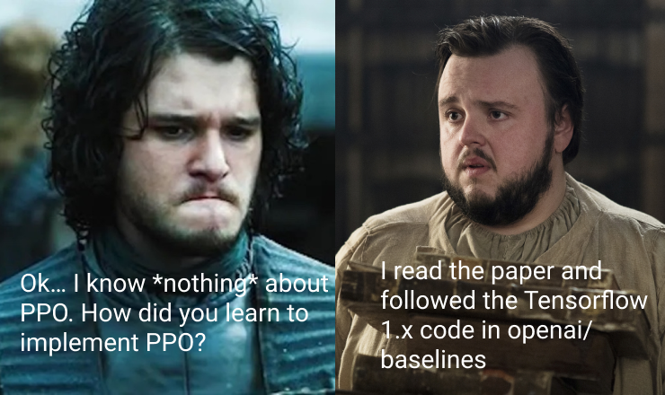
Jon is a first-year master’s student who is interested in reinforcement learning (RL). In his eyes, RL seemed fascinating because he could use RL libraries such as [Stable-Baselines3 (SB3)](https://github.com/DLR-RM/stable-baselines3) to train agents to play all kinds of games. He quickly recognized Proximal Policy Optimization (PPO) as a fast and versatile algorithm and wanted to implement PPO himself as a learning experience. Upon reading the paper, Jon thought to himself, “huh, this is pretty straightforward.” He then opened a code editor and started writing PPO. `CartPole-v1` from Gym was his chosen simulation environment, and before long, Jon made PPO work with `CartPole-v1`. He had a great time and felt motivated to make his PPO work with more interesting environments, such as the Atari games and MuJoCo robotics tasks. “How cool would that be?” he thought.
|
||
|
||
However, he soon struggled. Making PPO work with Atari and MuJoCo seemed more challenging than anticipated. Jon then looked for reference implementations online but was shortly overwhelmed: unofficial repositories all appeared to do things differently, whereas he just could not read the Tensorflow `1.x` code in the official repo. Fortunately, Jon stumbled across two recent papers that explain PPO’s implementations. “This is it!” he grinned. Failing to control his excitement, Jon started running around in the office, accidentally bumping into Sam, whom Jon knew was working on RL. They then had the following conversation:
|
||
|
||
* “Hey, I just read the _implementation details matter_ paper and the _what matters in on-policy RL_ paper. Fascinating stuff. I knew PPO wasn’t that easy!” Jon exclaimed.
|
||
* “Oh yeah! PPO is tricky, and I love these two papers that dive into the nitty-gritty details.” Sam answered.
|
||
* “Indeed. I feel I understand PPO much better now. You have been working with PPO, right? Quiz me on PPO!” Jon inquired enthusiastically.
|
||
* “Sure. If you run the official PPO with the Atari game Breakout, the agent would get ~400 game scores in about 4 hours. Do you know how does PPO achieve that?”
|
||
* “Hmm… That’s actually a good question. I don’t think the two papers explain that.”
|
||
* “The procgen paper contains experiments conducted using the official PPO with LSTM. Do you know how does PPO + LSTM work?”
|
||
* “Ehh… I haven’t read too much on PPO + LSTM” Jon admitted.
|
||
* “The official PPO also works with `MultiDiscrete` action space where you can use multiple discrete values to describe an action. Do you know how that works?”
|
||
* “…” Jon, speechless.
|
||
* “Lastly, if you have only the standard tools (e.g., `numpy, gym...`) and a neural network library (e.g., `torch, jax,...`), could you code up PPO from scratch?”
|
||
* “Ooof, I guess it’s going to be difficult. Prior papers analyzed PPO implementation details but didn’t show how these pieces are coded together. Also, I now realize their conclusions are in MuJoCo tasks and do not necessarily transfer to other games such as Atari. I feel sad now…” Jon sighed.
|
||
* “Don’t feel bad. PPO is just a complicated beast. If anything helps, I have been making video tutorials on implementing PPO from scratch and a blog post explaining things in more depth!”
|
||
|
||
|
||
|
||
And the blog post is here! Instead of doing ablation studies and making recommendations on which details matter, this blog post takes a step back and focuses on reproductions of PPO’s results in all accounts. Specifically, this blog post complements prior work in the following ways:
|
||
|
||
1. **Genealogy Analysis:** we establish what it means to reproduce the **official PPO implementation** by examining its historical revisions in the `openai/baselines` GitHub repository (the official repository for PPO). As we will show, the code in the `openai/baselines` repository has undergone several refactorings which could produce different results from the original paper. So it is important to recognize _which version_ of the official implementation is worth studying.
|
||
2. **Video Tutorials and Single-file Implementations:** we make video tutorials on re-implementing PPO in PyTorch from scratch, matching details in the official PPO implementation to handle classic control tasks, Atari games, and MuJoCo tasks. Notably, we adopt single-file implementations in our code base, making the code quicker and easier to read. The videos are shown below:
|
||
|
||
[Video 13](https://www.youtube.com/watch?v=MEt6rrxH8W4)[Video 14](https://www.youtube.com/watch?v=05RMTj-2K_Y)[Video 15](https://www.youtube.com/watch?v=BvZvx7ENZBw)
|
||
|
||
1. **Implementation Checklist with References:** During our re-implementation, we have compiled an implementation checklist containing 37 details as follows. For each implementation detail, we display the permanent link to its code (which is not done in academic papers) and point out its literature connection.
|
||
* 13 core implementation details
|
||
* 9 Atari specific implementation details
|
||
* 9 implementation details for robotics tasks (with continuous action spaces)
|
||
* 5 LSTM implementation details
|
||
* 1 `MultiDiscrete` action spaces implementation detail
|
||
|
||
2. **High-fidelity Reproduction:** To validate our re-implementation, we show that the empirical results of our implementation match closely with those of the original, in classic control tasks, Atari games, MuJoCo tasks, LSTM, and Real-time Strategy (RTS) game tasks.
|
||
3. **Situational Implementation Details:** We also cover 4 implementation details not used in the official implementation but potentially useful on special occasions.
|
||
|
||
Our ultimate purpose is to help people understand the PPO implementation through and through, reproduce past results with high fidelity, and facilitate customization for new research. To make research reproducible, we have made source code available at [https://github.com/vwxyzjn/ppo-implementation-details](https://github.com/vwxyzjn/ppo-implementation-details) and the tracked experiments available at [https://wandb.ai/vwxyzjn/ppo-details](https://wandb.ai/vwxyzjn/ppo-details)
|
||
|
||
## Background
|
||
|
||
PPO is a policy gradient algorithm proposed by [Schulman et al., (2017)](https://iclr-blog-track.github.io/2022/03/25/ppo-implementation-details/#Schulman2017). As a refinement to Trust Region Policy Optimization (TRPO) ([Schulman et al., 2015](https://iclr-blog-track.github.io/2022/03/25/ppo-implementation-details/#Schulman2015)), PPO uses a simpler clipped surrogate objective, omitting the expensive second-order optimization presented in TRPO. Despite this simpler objective, [Schulman et al., (2017)](https://iclr-blog-track.github.io/2022/03/25/ppo-implementation-details/#Schulman2017) show PPO has higher sample efficiency than TRPO in many control tasks. PPO also has good empirical performance in the arcade learning environment (ALE) which contain Atari games.
|
||
|
||
To facilitate more transparent research, [Schulman et al., (2017)](https://iclr-blog-track.github.io/2022/03/25/ppo-implementation-details/#Schulman2017) have made the source code of PPO available in the `openai/baselines` GitHub repository with the code name `pposgd` (commit [da99706](https://github.com/openai/baselines/tree/da997060461e3cbf54ca4dc7a67081a731fb6b3b/baselines/pposgd) on 7/20/2017). Later, the `openai/baselines` maintainers have introduced a series of revisions. The key events include:
|
||
|
||
1. 11/16/2017, commit [2dd7d30](https://github.com/openai/baselines/tree/2dd7d307d7d163a02b37c87c62b7949af02d99ad/baselines/ppo2): the maintainers introduced a refactored version `ppo2` and renamed `pposgd` to `ppo1`. According to a [GitHub issue](https://github.com/openai/baselines/issues/485#issuecomment-413722708), one maintainer suggests `ppo2` should offer better GPU utilization by batching observations from multiple simulation environments.
|
||
2. 8/10/2018, commit [ea68f3b](https://github.com/openai/baselines/commits/ea68f3b7e6a20d4c6bf1e32f8fb5ce18e6ef3a89): after a few revisions, the maintainers evaluated `ppo2`, producing the [MuJoCo benchmark](https://github.com/openai/baselines/blob/ea25b9e8b234e6ee1bca43083f8f3cf974143998/benchmarks_mujoco1M.htm)
|
||
3. 10/4/2018, commit [7bfbcf1](https://github.com/openai/baselines/commit/7bfbcf177eca8f46c0c0bfbb378e044539f5e061): after a few revisions, the maintainers evaluated `ppo2`, producing the [Atari benchmark](https://github.com/openai/baselines/blob/ea25b9e8b234e6ee1bca43083f8f3cf974143998/benchmarks_mujoco1M.htm)
|
||
4. 1/31/2020, commit [ea25b9e](https://github.com/openai/baselines/commit/ea25b9e8b234e6ee1bca43083f8f3cf974143998): the maintainers have merged the last commit to `openai/baselines` to date. To our knowledge, `ppo2` ([ea25b9e](https://github.com/openai/baselines/commit/ea25b9e8b234e6ee1bca43083f8f3cf974143998)) is the base of many PPO-related resources:
|
||
1. RL libraries such [Stable-Baselines3 (SB3)](https://github.com/DLR-RM/stable-baselines3), [pytorch-a2c-ppo-acktr-gail](https://github.com/ikostrikov/pytorch-a2c-ppo-acktr-gail), and [CleanRL](https://github.com/vwxyzjn/cleanrl) have built their PPO implementation to match implementation details in `ppo2` ([ea25b9e](https://github.com/openai/baselines/commit/ea25b9e8b234e6ee1bca43083f8f3cf974143998)) closely.
|
||
2. Recent papers ([Engstrom, Ilyas, et al., 2020](https://iclr-blog-track.github.io/2022/03/25/ppo-implementation-details/#Engstrom); [Andrychowicz, et al., 2021](https://iclr-blog-track.github.io/2022/03/25/ppo-implementation-details/#Andrychowicz)) have examined implementation details concerning robotics tasks in `ppo2` ([ea25b9e](https://github.com/openai/baselines/commit/ea25b9e8b234e6ee1bca43083f8f3cf974143998)).
|
||
|
||
In recent years, reproducing PPO’s results has become a challenging issue. The following table collects the best-reported performance of PPO in popular RL libraries in Atari and MuJoCo environments.
|
||
|
||
| RL Library | GitHub Stars | Benchmark Source | Breakout | Pong | BeamRider | Hopper | Walker2d | HalfCheetah |
|
||
| --- | --- | --- | --- | --- | --- | --- | --- | --- |
|
||
| [Baselines](https://github.com/openai/baselines)`pposgd` / `ppo1` ([da99706](https://github.com/openai/baselines/tree/da997060461e3cbf54ca4dc7a67081a731fb6b3b/baselines/pposgd)) | [](https://github.com/openai/baselines/stargazers) | [paper](https://arxiv.org/abs/1707.06347) ($) | 274.8 | 20.7 | 1590 | ~2250 | ~3000 | ~1750 |
|
||
| [Baselines](https://github.com/openai/baselines)`ppo2` ([7bfbcf1](https://github.com/openai/baselines/commit/7bfbcf177eca8f46c0c0bfbb378e044539f5e061) and [ea68f3b](https://github.com/openai/baselines/commits/ea68f3b7e6a20d4c6bf1e32f8fb5ce18e6ef3a89)) | | [docs](https://github.com/openai/baselines/blob/master/benchmarks_atari10M.htm) (*) | 114.26 | 13.68 | 1299.25 | 2316.16 | 3424.95 | 1668.58 |
|
||
| [Baselines](https://github.com/openai/baselines)`ppo2` ([ea25b9e](https://github.com/openai/baselines/commit/ea25b9e8b234e6ee1bca43083f8f3cf974143998)) | | this blog post (*) | 409.265 ± 30.98 | 20.59 ± 0.40 | 2627.96 ± 625.751 | 2448.73 ± 596.13 | 3142.24 ± 982.25 | 2148.77 ± 1166.023 |
|
||
| [Stable-Baselines3](https://github.com/DLR-RM/stable-baselines3) | [](https://github.com/DLR-RM/stable-baselines3/stargazers) | [docs](https://github.com/DLR-RM/rl-baselines3-zoo/blob/111d03c4ce728fff51d4b1c10355ea612bc8d456/benchmark.md) (0) (^) | 398.03 ± 33.28 | 20.98 ± 0.10 | 3397.00 ± 1662.36 | 2410.43 ± 10.02 | 3478.79 ± 821.70 | 5819.09 ± 663.53 |
|
||
| [CleanRL](https://github.com/vwxyzjn/cleanrl) | [](https://github.com/vwxyzjn/cleanrl/stargazers) | [docs](https://wandb.ai/cleanrl/cleanrl.benchmark/reports/Open-RL-Benchmark-0-6-0---Vmlldzo0MDcxOA) (1) (*) | ~402 | ~20.39 | ~2131 | ~2685 | ~3753 | ~1683 |
|
||
| [Tianshou](https://github.com/thu-ml/tianshou) | [](https://github.com/thu-ml/tianshou/stargazers) | [paper](https://arxiv.org/pdf/2107.14171.pdf), [docs](https://github.com/thu-ml/tianshou/blob/f13e415eb0de55baca5dc0d6fae39d6a38e8bc0b/examples/atari/README.md) (5) (^) | ~400 | ~20 | - | 7337.4 ± 1508.2 | 3127.7 ± 413.0 | 4895.6 ± 704.3 |
|
||
| [Ray/RLlib](https://github.com/ray-project/ray/tree/master/rllib/) | [](https://github.com/ray-project/ray/stargazers) | [repo](https://github.com/ray-project/rl-experiments/tree/9543891717cd0f8e137e23812229a06f8ed1c6c2) (2) (*) | 201 | - | 4480 | - | - | 9664 |
|
||
| [SpinningUp](https://github.com/openai/spinningup) | [](https://github.com/openai/spinningupstargazers) | [docs](https://spinningup.openai.com/en/latest/spinningup/bench.html#id12) (3) (^) | - | - | - | ~2500 | ~2500 | ~3000 |
|
||
| [ChainerRL](https://github.com/chainer/chainerrl) | [](https://github.com/chainer/chainerrl/stargazers) | [paper](https://arxiv.org/pdf/1912.03905.pdf) (4) (*) | - | - | - | 2719 ± 67 | 2994 ± 113 | 2404 ± 185 |
|
||
| [Tonic](https://github.com/fabiopardo/tonic) | [](https://github.com/fabiopardo/tonic/stargazers) | [paper](https://arxiv.org/pdf/2011.07537.pdf) (6) (^) | - | - | - | ~2000 | ~4500 | ~5000 |
|
||
|
||
(-): No publicly reported metrics available
|
||
|
||
($): The experiments uses the v1 MuJoCo environments
|
||
|
||
(*): The experiments uses the v2 MuJoCo environments
|
||
|
||
(^): The experiments uses the v3 MuJoCo environments
|
||
|
||
(0): 1M steps for MuJoCo experiments, 10M steps for Atari games, 1 random seed
|
||
|
||
(1): 2M steps for MuJoCo experiments, 10M steps for Atari games, 2 random seeds
|
||
|
||
(2): 25M steps and 10 workers (5 envs per worker) for Atari experiments; 44M steps and 16 workers for MuJoCo experiments; 1 random seed
|
||
|
||
(3): 3M steps, PyTorch version, 10 random seeds
|
||
|
||
(4): 2M steps, 10 random seeds
|
||
|
||
(5): 3M steps, 10 random seeds for MuJoCo experiments; 10M steps, 1 random seed for Atari experiment
|
||
|
||
(6): 5M steps, 10 random seeds
|
||
|
||
We offer several observations.
|
||
|
||
1. These revisions in `openai/baselines` are not without performance consequences. Reproducing PPO’s results is challenging partly because even the original implementation could produce inconsistent results.
|
||
2. `ppo2` ([ea25b9e](https://github.com/openai/baselines/commit/ea25b9e8b234e6ee1bca43083f8f3cf974143998)) and libraries matching its implementation details have reported rather similar results. In comparison, other libraries have usually reported more diverse results.
|
||
3. Interestingly, we have found many libraries reported performance in MuJoCo tasks but not in Atari tasks.
|
||
|
||
Despite the complicated situation, we have found `ppo2` ([ea25b9e](https://github.com/openai/baselines/commit/ea25b9e8b234e6ee1bca43083f8f3cf974143998)) as an implementation worth studying. It obtains good performance in both Atari and MuJoCo tasks. More importantly, it also incorporates advanced features such as LSTM and treatment of the `MultiDiscrete` action space, unlocking application to more complicated games such as Real-time Strategy games. As such, we define `ppo2` ([ea25b9e](https://github.com/openai/baselines/commit/ea25b9e8b234e6ee1bca43083f8f3cf974143998)) as the **official PPO implementation** and base the remainder of this blog post on this implementation.
|
||
|
||
## Reproducing the official PPO implementation
|
||
|
||
In this section, we introduce five categories of implementation details and implement them in PyTorch from scratch.
|
||
|
||
* 13 core implementation details
|
||
* 9 Atari specific implementation details
|
||
* 9 implementation details for robotics tasks (with continuous action spaces)
|
||
* 5 LSTM implementation details
|
||
* 1 `MultiDiscrete` implementation detail
|
||
|
||
For each category (except the first one), we benchmark our implementation against the original implementation in three environments, each with three random seeds.
|
||
|
||
## 13 core implementation details
|
||
|
||
We first introduce the 13 core implementation details commonly used regardless of the tasks. To help understand how to code these details in PyTorch, we have prepared a line-by-line video tutorial as follows. Note that the video tutorial skips over the 12-th and 13-th implementation details during its making, hence the video has the title “11 Core Implementation Details”
|
||
|
||
[Video 16](https://www.youtube.com/watch?v=MEt6rrxH8W4)
|
||
|
||
1. Vectorized architecture ([common/cmd_util.py#L22](https://github.com/openai/baselines/blob/ea25b9e8b234e6ee1bca43083f8f3cf974143998/baselines/common/cmd_util.py#L22)) Code-level Optimizations
|
||
* PPO leverages an efficient paradigm known as the **vectorized architecture** that features a single learner that collects samples and learns from multiple environments. Below is a pseudocode: ```
|
||
envs = VecEnv(num_envs=N)
|
||
agent = Agent()
|
||
next_obs = envs.reset()
|
||
next_done = [0, 0, ..., 0] # of length N
|
||
for update in range(1, total_timesteps // (N*M)):
|
||
data = []
|
||
# ROLLOUT PHASE
|
||
for step in range(0, M):
|
||
obs = next_obs
|
||
done = next_done
|
||
action, other_stuff = agent.get_action(obs)
|
||
next_obs, reward, next_done, info = envs.step(
|
||
action
|
||
) # step in N environments
|
||
data.append([obs, action, reward, done, other_stuff]) # store data
|
||
|
||
# LEARNING PHASE
|
||
agent.learn(data, next_obs, next_done) # `len(data) = N*M`
|
||
```
|
||
* In this architecture, PPO first initializes a **vectorized environment**`envs` that runs $N$ (usually independent) environments either sequentially or in parallel by leveraging multi-processes. `envs` presents a synchronous interface that always outputs a batch of $N$ observations from $N$ environments, and it takes a batch of $N$ actions to step the $N$ environments. When calling `next_obs = envs.reset()`, `next_obs` gets a batch of $N$ initial observations (pronounced “next observation”). PPO also initializes an environment done flag variable `next_done` (pronounced “next done”) to an $N$-length array of zeros, where its i-th element `next_done[i]` has values of 0 or 1 which corresponds to the $i$-th sub-environment being _not done_ and _done_, respectively.
|
||
* Then, the vectorized architecture loops two phases: the **rollout phase** and the **learning phase**:
|
||
* Rollout phase : The agent samples actions for the $N$ environments and continue to step them for a fixed number of $M$ steps. During these $M$ steps, the agent continues to append relevant data in an empty list `data`. If the $i$-th sub-environment is done (terminated or truncated) after stepping with the $i$-th action `action[i]`, `envs` would set its returned `next_done[i]` to 1, auto-reset the $i$-th sub-environment and fill `next_obs[i]` with the initial observation in the new episode of the $i$-th environment.
|
||
* Learning phase: The agent in principal learns from the collected data in the rollout phase: `data` of length $N M$, `next_obs` and `done`. Specifically, PPO can estimate value for the next observation `next_obs` conditioned on `next_done` and calculate the advantage `advantages` and the return `returns`, both of which also has length $N M$. PPO then learns from the prepared data `[data, advantages, returns]`, which is called “fixed-length trajectory segments” by [(Schulman et al., 2017)](https://iclr-blog-track.github.io/2022/03/25/ppo-implementation-details/#Schulman2017).
|
||
* **It is important to understand `next_obs` and `next_done`’s role to help transition between phases**: At the end of the $j$-th rollout phase, `next_obs` can be used to estimate the value of the final state during learning phase, and in the begining of the $\left(\right. j + 1 \left.\right)$-th rollout phase, `next_obs` becomes the initial observation in `data`. Likewise, `next_done` tells if `next_obs` is actually the first observation of a new episode. This intricate design allows PPO to continue step the sub-environments, and because agent always learns from fixed-length trajectory segments after $M$ steps, PPO can train the agent even if the sub-environments never terminate or truncate. This is in principal why PPO can learn in long-horizon games that last 100,000 steps [(default truncation limit for Atari games in `gym`)](https://github.com/openai/gym/blob/a7b6462136ebaa610c8941e4da8a9c92155b04d1/gym/envs/__init__.py#L744) in a single episode.
|
||
|
||
* A common incorrect implementation is to train PPO based on episodes and setting a maximum episode horizon. Below is a pseudocode. ```
|
||
env = Env()
|
||
agent = Agent()
|
||
for episode in range(1, num_episodes):
|
||
next_obs = env.reset()
|
||
data = []
|
||
for step in range(1, max_episode_horizon):
|
||
obs = next_obs
|
||
action, other_stuff = agent.get_action(obs)
|
||
next_obs, reward, done, info = env.step(action)
|
||
data.append([obs, action, reward, done, other_stuff]) # store data
|
||
if done:
|
||
break
|
||
agent.learn(data)
|
||
```
|
||
* There are several downsides to this approach. First, it can be inefficient because the agent has to do one forward pass per environment step. Second, it does not scale to games with larger horizons such as StarCraft II (SC2). A single episode of the SC2 could last 100,000 steps, which bloats the memory requirement in this implementation.
|
||
* The vectorized architecture handles this 100,000 steps by learning from **fixed-length trajectory segments**. If we set $N = 2$ and $M = 100$, the agent would learn from the first 100 steps from 2 independent environments. Then, note that the `next_obs` is the 101st observation from these two environments, and the agent can keep doing rollouts and learn from the 101 to 200 steps from the 2 environments. Essentially, the agent learns partial trajectories of the episode, $M$ steps at a time.
|
||
|
||
* $N$ is the `num_envs` (decision C1) and $M * N$ is the `iteration_size` (decision C2) in [Andrychowicz, et al. (2021)](https://iclr-blog-track.github.io/2022/03/25/ppo-implementation-details/#Andrychowicz), who suggest increasing $N$ (such as $N = 256$) boosts the training throughput but makes the performance worse. They argued the performance deterioration was due to “shortened experience chunks” ($M$ becomes smaller due to the increase in $N$ in their setup ) and “earlier value bootstrapping.” While we agree increasing $N$ could hurt sample efficiency, we argue the evaluation should be based on wall-clock time efficiency. That is, if the algorithm terminates much sooner with a larger $N$ compared to other configurations, why not run the algorithm longer? Although being a different robotics simulator, [Brax](https://github.com/google/brax) follows this idea and can train a viable agent in similar tasks with PPO using a massive $N = 2048$ and a small $M = 20$ yet finish the training in one minute.
|
||
* The vectorized environments also support multi-agent reinforcement learning (MARL) environments. Below is the quote from ([gym3](https://github.com/openai/gym3)) using our notation:
|
||
> In the simplest case, a vectorized environment corresponds to a single multiplayer game with $N$ players. If we run an RL algorithm in this environment, we are doing self-play without historical opponents. This setup can be straightforwardly extended to having $K$ concurrent games with $H$ players each, with $N = H * K$.
|
||
|
||
* For example, if there is a two-player game, we can create a vectorized environment that spawns two sub-environments. Then, the vectorized environment produces a batch of two observations, where the first observation is from player 1 and the second observation is from player 2. Next, the vectorized environment takes a batch of two actions and tells the game engine to let player 1 execute the first action and player 2 execute the second action. Consequently, PPO learns to control both player 1 and player 2 in this vectorized environment.
|
||
* Such MARL usage is widely adopted in games such as Gym-μRTS ([Huang et al, 2021](https://iclr-blog-track.github.io/2022/03/25/ppo-implementation-details/#Huang2021)), Pettingzoo ([Terry et al, 2021](https://iclr-blog-track.github.io/2022/03/25/ppo-implementation-details/#Terry)), etc.
|
||
|
||
2. Orthogonal Initialization of Weights and Constant Initialization of biases ([a2c/utils.py#L58)](https://github.com/openai/baselines/blob/ea25b9e8b234e6ee1bca43083f8f3cf974143998/baselines/a2c/utils.py#L58)) Neural Network Code-level Optimizations
|
||
* The related code is across multiple files in the `openai/baselines` library. The code for such initialization is in [a2c/utils.py#L58](https://github.com/openai/baselines/blob/ea25b9e8b234e6ee1bca43083f8f3cf974143998/baselines/a2c/utils.py#L58), when in fact it is used for other algorithms such as PPO. In general, the weights of _hidden_ layers use orthogonal initialization of weights with scaling `np.sqrt(2)`, and the biases are set to `0`, as shown in the CNN initialization for Atari ([common/models.py#L15-L26](https://github.com/openai/baselines/blob/ea25b9e8b234e6ee1bca43083f8f3cf974143998/baselines/common/models.py#L15-L26)), and the MLP initialization for Mujoco ([common/models.py#L75-L103](https://github.com/openai/baselines/blob/ea25b9e8b234e6ee1bca43083f8f3cf974143998/baselines/common/models.py#L75-L103)). However, the policy output layer weights are initialized with the scale of `0.01`. The value output layer weights are initialized with the scale of `1` ([common/policies.py#L49-L63](https://github.com/openai/baselines/blob/ea25b9e8b234e6ee1bca43083f8f3cf974143998/baselines/common/policies.py#L49-L63)).
|
||
* It seems the implementation of the orthogonal initialization of `openai/baselines` ([a2c/utils.py#L20-L35](https://github.com/openai/baselines/blob/ea25b9e8b234e6ee1bca43083f8f3cf974143998/baselines/a2c/utils.py#L20-L35)) is different from that of pytorch/pytorch ([torch.nn.init.orthogonal_](https://pytorch.org/docs/stable/_modules/torch/nn/init.html#orthogonal_)). However, we consider this to be a very low-level detail that should not impact the performance.
|
||
* [Engstrom, Ilyas, et al., (2020)](https://iclr-blog-track.github.io/2022/03/25/ppo-implementation-details/#Engstrom) find orthogonal initialization to outperform the default Xavier initialization in terms of the highest episodic return achieved. Also, [Andrychowicz, et al. (2021)](https://iclr-blog-track.github.io/2022/03/25/ppo-implementation-details/#Andrychowicz) find centering the action distribution around 0 (i.e., initialize the policy output layer weights with 0.01”) to be beneficial (decision C57).
|
||
|
||
3. The Adam Optimizer’s Epsilon Parameter ([ppo2/model.py#L100](https://github.com/openai/baselines/blob/ea25b9e8b234e6ee1bca43083f8f3cf974143998/baselines/ppo2/model.py#L100)) Code-level Optimizations
|
||
* PPO sets the epsilon parameter to `1e-5`, which is different from the default epsilon of `1e-8` in PyTorch and `1e-7` in TensorFlow. We list this implementation detail because the epsilon parameter is neither mentioned in the paper nor a configurable parameter in the PPO implementation. While this implementation detail may seem over specific,it is important that we match it for a high-fidelity reproduction.
|
||
* [Andrychowicz, et al. (2021)](https://iclr-blog-track.github.io/2022/03/25/ppo-implementation-details/#Andrychowicz) perform a grid search on Adam optimizer’s parameters (decision C24, C26, C28) and recommend $\beta_{1} = 0.9$ and use the Tensorflow’s default epsilon parameter `1e-7`. [Engstrom, Ilyas, et al., (2020)](https://iclr-blog-track.github.io/2022/03/25/ppo-implementation-details/#Engstrom) use the default PyTorch epsilon parameter `1e-8`.
|
||
|
||
4. Adam Learning Rate Annealing ([ppo2/ppo2.py#L133-L135](https://github.com/openai/baselines/blob/ea25b9e8b234e6ee1bca43083f8f3cf974143998/baselines/ppo2/ppo2.py#L133-L135)) Code-level Optimizations
|
||
* The Adam optimizer’s learning rate could be either constant or set to decay. By default, the hyper-parameters for training agents playing Atari games set the learning rate to linearly decay from `2.5e-4` to `0` as the number of timesteps increases. In MuJoCo, the learning rate linearly decays from `3e-4` to `0`.
|
||
* [Engstrom, Ilyas, et al., (2020)](https://iclr-blog-track.github.io/2022/03/25/ppo-implementation-details/#Engstrom) find adam learning rate annealing to help agents obtain higher episodic return. Also, [Andrychowicz, et al. (2021)](https://iclr-blog-track.github.io/2022/03/25/ppo-implementation-details/#Andrychowicz) have also found learning rate annealing helpful as it increases performance in 4 out of 5 tasks examined, although the performance gains are relatively small (decision C31, figure 65).
|
||
|
||
5. Generalized Advantage Estimation ([ppo2/runner.py#L56-L65](https://github.com/openai/baselines/blob/ea25b9e8b234e6ee1bca43083f8f3cf974143998/baselines/ppo2/runner.py#L56-L65)) Theory
|
||
* Although the PPO paper uses the abstraction of advantage estimate in the PPO’s objective, the PPO implementation does use Generalized Advantage Estimation ([Schulman, 2015b](https://iclr-blog-track.github.io/2022/03/25/ppo-implementation-details/#Schulman2015b)). Two important sub-details:
|
||
* Value bootstrap ([ppo2/runner.py#L50](https://github.com/openai/baselines/blob/ea25b9e8b234e6ee1bca43083f8f3cf974143998/baselines/ppo2/runner.py#L50)): if a sub-environment is _not_ terminated nor truncated, PPO estimates the value of the next state in this sub-environment as the value target.
|
||
* **A note on truncation**: Almost all `gym` environments have a time limit and will truncate themselves if they run too long. For example, the `CartPole-v1` has a 500 time limit (see [link](https://github.com/openai/gym/blob/e9df4932434516c9f7956cc8010679a33835b204/gym/envs/__init__.py#L26)) and will return `done=True` if the game lasts for more than 500 steps. While the PPO implementation does not estimate value of the terminal state in the truncated environments, we (intuitively) should. Nonetheless, for high-fidelity reproduction, we did not implement the correct handling for truncated environments.
|
||
|
||
* $T D \left(\right. \lambda \left.\right)$ return estimation ([ppo2/runner.py#L65](https://github.com/openai/baselines/blob/ea25b9e8b234e6ee1bca43083f8f3cf974143998/baselines/ppo2/runner.py#L65)): PPO implements the return target as `returns = advantages + values`, which corresponds to $T D \left(\right. \lambda \left.\right)$ for value estimation (where Monte Carlo estimation is a special case when $\lambda = 1$).
|
||
|
||
* [Andrychowicz, et al. (2021)](https://iclr-blog-track.github.io/2022/03/25/ppo-implementation-details/#Andrychowicz) find GAE to performan better than N-step returns (decision C6, figure 44 and 40).
|
||
|
||
6. Mini-batch Updates ([ppo2/ppo2.py#L157-L166](https://github.com/openai/baselines/blob/ea25b9e8b234e6ee1bca43083f8f3cf974143998/baselines/ppo2/ppo2.py#L157-L166)) Code-level Optimizations
|
||
* During the learning phase of the vectorized architecture, the PPO implementation shuffles the indices of the training data of size $N * M$ and breaks it into mini-batches to compute the gradient and update the policy.
|
||
* Some common mis-implementations include 1) always using the whole batch for the update, and 2) implementing mini-batches by randomly fetching from the training data (which does not guarantee all training data points are fetched).
|
||
|
||
7. Normalization of Advantages ([ppo2/model.py#L139](https://github.com/openai/baselines/blob/ea25b9e8b234e6ee1bca43083f8f3cf974143998/baselines/ppo2/model.py#L139)) Code-level Optimizations
|
||
* After calculating the advantages based on GAE, PPO normalizes the advantages by subtracting their mean and dividing them by their standard deviation. In particular, _this normalization happens at the minibatch level instead of the whole batch level!_
|
||
* [Andrychowicz, et al. (2021)](https://iclr-blog-track.github.io/2022/03/25/ppo-implementation-details/#Andrychowicz) (decision C67) find per-minibatch advantage normalization to not affect performance much (figure 35).
|
||
|
||
8. Clipped surrogate objective ([ppo2/model.py#L81-L86](https://github.com/openai/baselines/blob/ea25b9e8b234e6ee1bca43083f8f3cf974143998/baselines/ppo2/model.py#L81-L86)) Theory
|
||
* PPO clips the objective as suggested in the paper.
|
||
* [Engstrom, Ilyas, et al., (2020)](https://iclr-blog-track.github.io/2022/03/25/ppo-implementation-details/#Engstrom) find the PPO’s clipped objective to have similar performance to TRPO’s objective when they controlled other implementation details to be the same. [Andrychowicz, et al. (2021)](https://iclr-blog-track.github.io/2022/03/25/ppo-implementation-details/#Andrychowicz) find the PPO’s clipped objective to outperform vanilla policy gradient (PG), V-trace, AWR, and V-MPO in most tasks ([Espeholt et al., 2018](https://iclr-blog-track.github.io/2022/03/25/ppo-implementation-details/#IMPALA)).
|
||
* Based on the above findings, we argue PPO’s clipped objective is still a great objective because it achieves similar performance as TRPO’s objective while being computationally cheaper (i.e., without second order optimization as does in TRPO).
|
||
|
||
9. Value Function Loss Clipping ([ppo2/model.py#L68-L75](https://github.com/openai/baselines/blob/ea25b9e8b234e6ee1bca43083f8f3cf974143998/baselines/ppo2/model.py#L68-L75)) Code-level Optimizations
|
||
* PPO clips the value function like the PPO’s clipped surrogate objective. Given the `V_{targ} = returns = advantages + values`, PPO fits the the value network by minimizing the following loss:
|
||
|
||
$$
|
||
L^{V} = max \left[\right. \left(\left(\right. V_{\theta_{t}} - V_{t a r g} \left.\right)\right)^{2} , \left(\left(\right. clip \left(\right. V_{\theta_{t}} , V_{\theta_{t - 1}} - \epsilon , V_{\theta_{t - 1}} + \epsilon \left.\right) - V_{t a r g} \left.\right)\right)^{2} \left]\right.
|
||
$$
|
||
|
||
* [Engstrom, Ilyas, et al., (2020)](https://iclr-blog-track.github.io/2022/03/25/ppo-implementation-details/#Engstrom) find no evidence that the value function loss clipping helps with the performance. [Andrychowicz, et al. (2021)](https://iclr-blog-track.github.io/2022/03/25/ppo-implementation-details/#Andrychowicz) suggest value function loss clipping even hurts performance (decision C13, figure 43).
|
||
* We implemented this detail because this work is more about high-fidelity reproduction of prior results.
|
||
|
||
10. Overall Loss and Entropy Bonus ([ppo2/model.py#L91](https://github.com/openai/baselines/blob/ea25b9e8b234e6ee1bca43083f8f3cf974143998/baselines/ppo2/model.py#L91)) Theory
|
||
* The overall loss is calculated as `loss = policy_loss - entropy * entropy_coefficient + value_loss * value_coefficient`, which maximizes an entropy bonus term. Note that the policy parameters and value parameters share the same optimizer.
|
||
* Mnih et al. have reported this entropy bonus to improve exploration by encouraging the action probability distribution to be slightly more random.
|
||
* [Andrychowicz, et al. (2021)](https://iclr-blog-track.github.io/2022/03/25/ppo-implementation-details/#Andrychowicz) overall find no evidence that the entropy term improves performance on continuous control environments (decision C13, figure 76 and 77).
|
||
|
||
11. Global Gradient Clipping ([ppo2/model.py#L102-L108](https://github.com/openai/baselines/blob/ea25b9e8b234e6ee1bca43083f8f3cf974143998/baselines/ppo2/model.py#L102-L108)) Code-level Optimizations
|
||
* For each update iteration in an epoch, PPO rescales the gradients of the policy and value network so that the “global l2 norm” (i.e., the norm of the concatenated gradients of all parameters) does not exceed `0.5`.
|
||
* [Andrychowicz, et al. (2021)](https://iclr-blog-track.github.io/2022/03/25/ppo-implementation-details/#Andrychowicz) find global gradient clipping to offer a small performance boost (decision C68, figure 34).
|
||
|
||
12. Debug variables ([ppo2/model.py#L115-L116](https://github.com/openai/baselines/blob/ea25b9e8b234e6ee1bca43083f8f3cf974143998/baselines/ppo2/model.py#L115-L116))
|
||
* The PPO implementation comes with several debug variables, which are
|
||
1. `policy_loss`: the mean policy loss across all data points.
|
||
2. `value_loss`: the mean value loss across all data points.
|
||
3. `entropy_loss`: the mean entropy value across all data points.
|
||
4. `clipfrac`: the fraction of the training data that triggered the clipped objective.
|
||
5. `approxkl`: the approximate Kullback–Leibler divergence, measured by `(-logratio).mean()`, which corresponds to the `k1` estimator in John Schulman’s blog post on [approximating KL divergence](http://joschu.net/blog/kl-approx.html). This blog post also suggests using an alternative estimator `((ratio - 1) - logratio).mean()`, which is unbiased and has less variance.
|
||
|
||
13. Shared and separate MLP networks for policy and value functions ([common/policies.py#L156-L160](https://github.com/openai/baselines/blob/ea25b9e8b234e6ee1bca43083f8f3cf974143998/baselines/common/policies.py#L156-L160), [baselines/common/models.py#L75-L103](https://github.com/openai/baselines/blob/ea25b9e8b234e6ee1bca43083f8f3cf974143998/baselines/common/models.py#L75-L103))Neural Network Code-level Optimizations
|
||
* By default, PPO uses a simple MLP network consisting of two layers of 64 neurons and Hyperbolic Tangent as the activation function. Then PPO builds a policy head and value head that share the outputs of the MLP network. Below is a pseudocode: ```
|
||
network = Sequential(
|
||
layer_init(Linear(np.array(envs.single_observation_space.shape).prod(), 64)),
|
||
Tanh(),
|
||
layer_init(Linear(64, 64)),
|
||
Tanh(),
|
||
)
|
||
value_head = layer_init(Linear(64, 1), std=1.0)
|
||
policy_head = layer_init(Linear(64, envs.single_action_space.n), std=0.01)
|
||
hidden = network(observation)
|
||
value = value_head(hidden)
|
||
action = Categorical(policy_head(hidden)).sample()
|
||
```
|
||
* Alternatively, PPO could build a policy function and a value function using separate networks by toggling the `value_network='copy'` argument. Then the pseudocode looks like this: ```
|
||
value_network = Sequential(
|
||
layer_init(Linear(np.array(envs.single_observation_space.shape).prod(), 64)),
|
||
Tanh(),
|
||
layer_init(Linear(64, 64)),
|
||
Tanh(),
|
||
layer_init(Linear(64, 1), std=1.0),
|
||
)
|
||
policy_network = Sequential(
|
||
layer_init(Linear(np.array(envs.single_observation_space.shape).prod(), 64)),
|
||
Tanh(),
|
||
layer_init(Linear(64, 64)),
|
||
Tanh(),
|
||
layer_init(Linear(64, envs.single_action_space.n), std=0.01),
|
||
)
|
||
value = value_network(observation)
|
||
action = Categorical(policy_network(observation)).sample()
|
||
```
|
||
|
||
We incorporate the first 12 details and the **separate-networks architecture** to produce a self-contained `ppo.py` ([link](https://github.com/vwxyzjn/ppo-implementation-details/blob/main/ppo.py)) that has 322 lines of code. Then, we make about [10 lines of code](https://www.diffchecker.com/07TdfFlg) change to adopt the **shared-network architecture**, resulting in a self-contained `ppo_shared.py` ([link](https://github.com/vwxyzjn/ppo-implementation-details/blob/main/ppo_shared.py)) that has 317 lines of code. The following shows the file difference between the `ppo.py` (left) and `ppo_shared.py` (right).
|
||
|
||
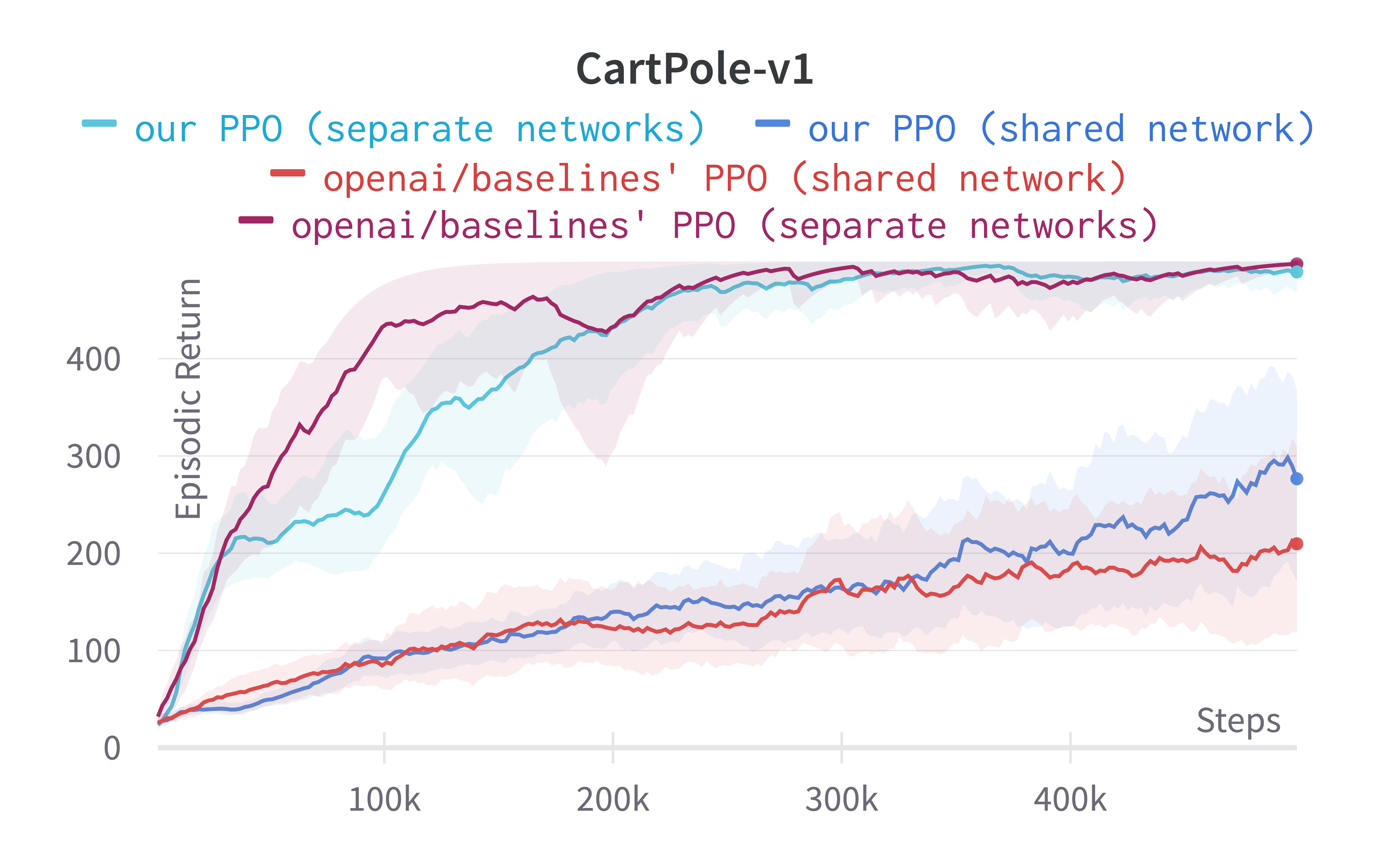
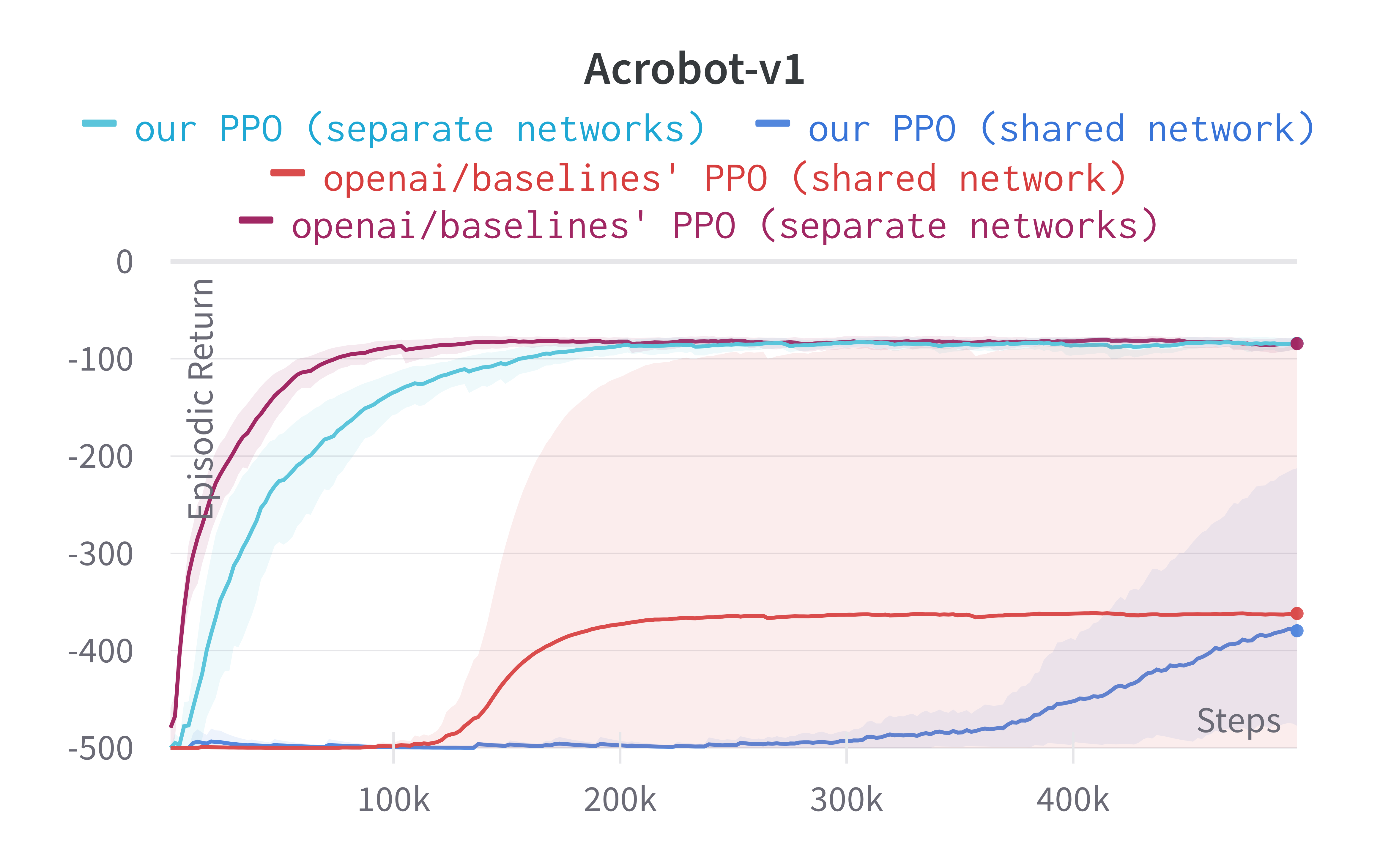
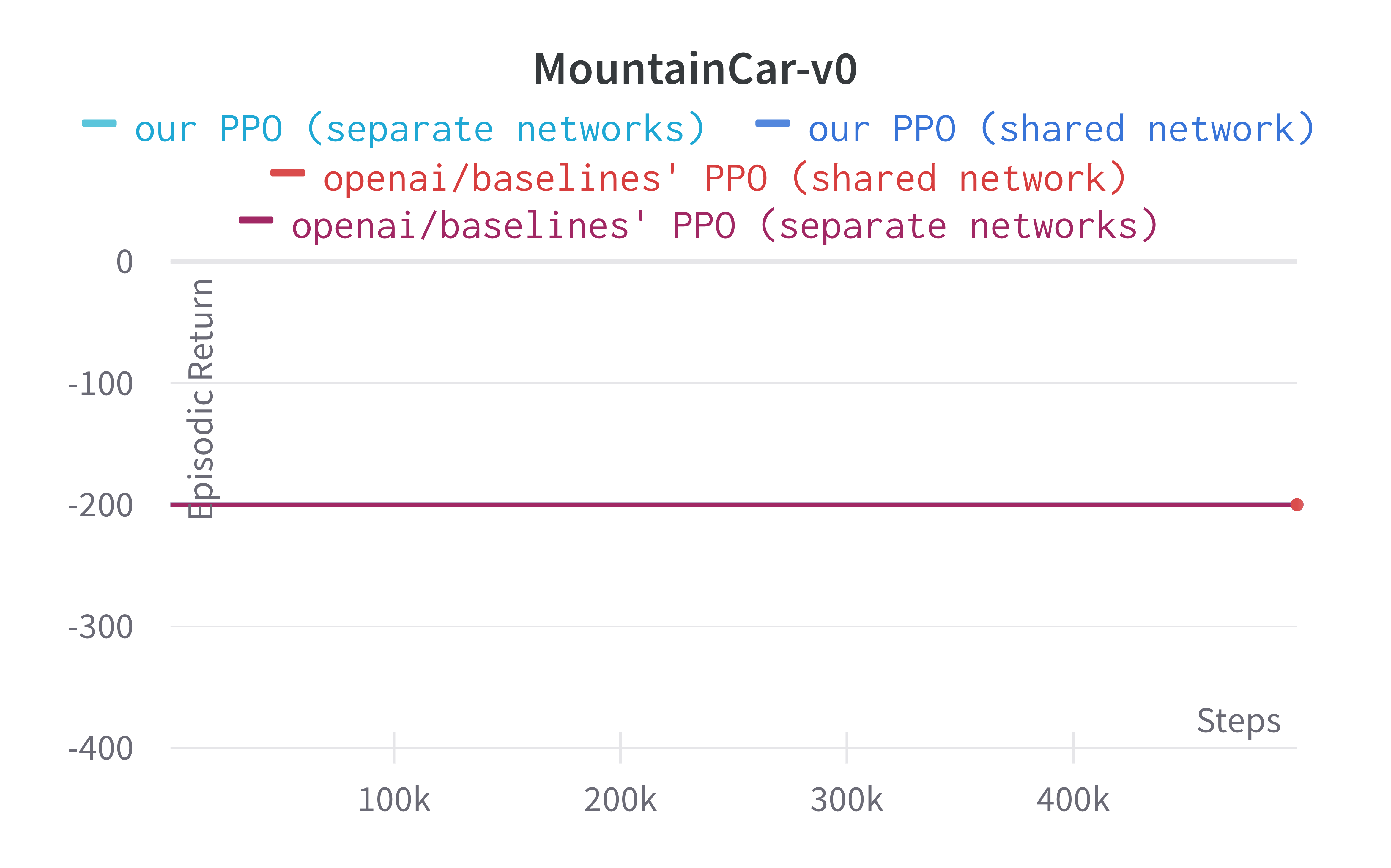
Below are the benchmarked results.
|
||
|
||
|
||
|
||
> Tracked classic control experiments (click to show the interactive panel)
|
||
|
||
While shared-network architecture is the default setting in PPO, the separate-networks architecture clearly outperforms in simpler environments. The shared-network architecture performs worse probably due to the competing objectives of the policy and value functions. For this reason, we implement the separate-networks architecture in the video tutorial.
|
||
|
||
## 9 Atari-specific implementation details
|
||
|
||
Next, we introduce the 9 Atari-specific implementation details. To help understand how to code these details in PyTorch, we have prepared a line-by-line video tutorial.
|
||
|
||
[Video 17](https://www.youtube.com/watch?v=05RMTj-2K_Y)
|
||
|
||
1. The Use of `NoopResetEnv` ([common/atari_wrappers.py#L12](https://github.com/openai/baselines/blob/ea25b9e8b234e6ee1bca43083f8f3cf974143998/baselines/common/atari_wrappers.py#L12)) Environment Preprocessing
|
||
* This wrapper samples initial states by taking a random number (between 1 and 30) of no-ops on reset.
|
||
* The source of this wrapper comes from [(Mnih et al., 2015, Extended Data Table 1)](https://iclr-blog-track.github.io/2022/03/25/ppo-implementation-details/#Mnih2015) and [Machado et al., 2018)](https://iclr-blog-track.github.io/2022/03/25/ppo-implementation-details/#Machado2018) have suggested `NoopResetEnv` is a way to inject stochasticity to the environment.
|
||
|
||
2. The Use of `MaxAndSkipEnv` ([common/atari_wrappers.py#L97](https://github.com/openai/baselines/blob/ea25b9e8b234e6ee1bca43083f8f3cf974143998/baselines/common/atari_wrappers.py#L97)) Environment Preprocessing
|
||
* This wrapper skips 4 frames by default, repeats the agent’s last action on the skipped frames, and sums up the rewards in the skipped frames. Such frame-skipping technique could considerably speed up the algorithm because the environment step is computationally cheaper than the agent’s forward pass [(Mnih et al., 2015)](https://iclr-blog-track.github.io/2022/03/25/ppo-implementation-details/#Mnih2015).
|
||
* This wrapper also returns the maximum pixel values over the last two frames to help deal with some Atari game quirks [(Mnih et al., 2015)](https://iclr-blog-track.github.io/2022/03/25/ppo-implementation-details/#Mnih2015).
|
||
* The source of this wrapper comes from [(Mnih et al., 2015)](https://iclr-blog-track.github.io/2022/03/25/ppo-implementation-details/#Mnih2015) as shown by the quote below.
|
||
> More precisely, the agent sees and selects actions on every $k$-th frame instead of every frame, and its last action is repeated on skipped frames. Because running the emulator forward for one step requires much less computation than having the agent select an action, this technique allows the agent to play roughly $k$ times more games without significantly increasing the runtime. We use $k = 4$ for all games. […] First, to encode a single frame we take the maximum value for each pixel color value over the frame being encoded and the previous frame. This was necessary to remove flickering that is present in games where some objects appear only in even frames while other objects appear only in odd frames, an artifact caused by the limited number of sprites Atari 2600 can display at once.
|
||
|
||
3. The Use of `EpisodicLifeEnv` ([common/atari_wrappers.py#L61](https://github.com/openai/baselines/blob/ea25b9e8b234e6ee1bca43083f8f3cf974143998/baselines/common/atari_wrappers.py#L61)) Environment Preprocessing
|
||
* In the games where there are a life counter such as breakout, this wrapper marks the end of life as the end of episode.
|
||
* The source of this wrapper comes from [(Mnih et al., 2015)](https://iclr-blog-track.github.io/2022/03/25/ppo-implementation-details/#Mnih2015) as shown by the quote below.
|
||
> For games where there is a life counter, the Atari 2600 emulator also sends the number of lives left in the game, which is then used to mark the end of an episode during training.
|
||
|
||
* Interestingly, [(Bellemare et al., 2016)](https://iclr-blog-track.github.io/2022/03/25/ppo-implementation-details/Bellemare2016b) Note this the wrapper could be detrimental to the agent’s performance and [Machado et al., 2018)](https://iclr-blog-track.github.io/2022/03/25/ppo-implementation-details/#Machado2018) have suggested not using this wrapper.
|
||
|
||
4. The Use of `FireResetEnv` ([common/atari_wrappers.py#L41](https://github.com/openai/baselines/blob/ea25b9e8b234e6ee1bca43083f8f3cf974143998/baselines/common/atari_wrappers.py#L41)) Environment Preprocessing
|
||
* This wrapper takes the `FIRE` action on reset for environments that are fixed until firing.
|
||
* This wrapper is interesting because there is no literature reference to our knowledge. According to anecdotal conversations([openai/baselines#240](https://github.com/openai/baselines/issues/240)), neither people from DeepMind nor OpenAI know where this wrapper comes from. So… 
|
||
|
||
5. The Use of `WarpFrame` (Image transformation) [common/atari_wrappers.py#L134](https://github.com/openai/baselines/blob/ea25b9e8b234e6ee1bca43083f8f3cf974143998/baselines/common/atari_wrappers.py#L134)Environment Preprocessing
|
||
* This wrapper warps extracts the Y channel of the 210x160 pixel images and resizes it to 84x84.
|
||
* The source of this wrapper comes from [(Mnih et al., 2015)](https://iclr-blog-track.github.io/2022/03/25/ppo-implementation-details/#Mnih2015) as shown by the quote below.
|
||
> Second, we then extract the Y channel, also known as luminance, from the RGB frame and rescale it to 84x84.
|
||
|
||
* In our implementation, we use the following wrappers to achieve the same purpose. ```
|
||
env = gym.wrappers.ResizeObservation(env, (84, 84))
|
||
env = gym.wrappers.GrayScaleObservation(env)
|
||
```
|
||
|
||
6. The Use of `ClipRewardEnv` ([common/atari_wrappers.py#L125](https://github.com/openai/baselines/blob/ea25b9e8b234e6ee1bca43083f8f3cf974143998/baselines/common/atari_wrappers.py#L125)) Environment Preprocessing
|
||
* This wrapper bins reward to `{+1, 0, -1}` by its sign.
|
||
* The source of this wrapper comes from [(Mnih et al., 2015)](https://iclr-blog-track.github.io/2022/03/25/ppo-implementation-details/#Mnih2015) as shown by the quote below.
|
||
> As the scale of scores varies greatly from game to game, we clipped all positive rewards at 1 and all negative rewards at -1, leaving 0 rewards unchanged. Clipping the rewards in this manner limits the scale of the error derivatives and makes it easier to use the same learning rate across multiple games. At the same time, it could affect the performance of our agent since it cannot differentiate between rewards of different magnitude.
|
||
|
||
7. The Use of `FrameStack` ([common/atari_wrappers.py#L188](https://github.com/openai/baselines/blob/ea25b9e8b234e6ee1bca43083f8f3cf974143998/baselines/common/atari_wrappers.py#L188)) Environment Preprocessing
|
||
* This wrapper stacks $m$ last frames such that the agent can infer the velocity and directions of moving objects.
|
||
* The source of this wrapper comes from [(Mnih et al., 2015)](https://iclr-blog-track.github.io/2022/03/25/ppo-implementation-details/#Mnih2015) as shown by the quote below.
|
||
> The function $\theta$ from algorithm 1 described below applies this preprocessing to the $m$ most recent frames and stacks them to produce the input to the Q-function, in which $m = 4$.
|
||
|
||
8. Shared Nature-CNN network for the policy and value functions ([common/policies.py#L157](https://github.com/openai/baselines/blob/ea25b9e8b234e6ee1bca43083f8f3cf974143998/baselines/common/policies.py#L157), [common/models.py#L15-L26](https://github.com/openai/baselines/blob/ea25b9e8b234e6ee1bca43083f8f3cf974143998/baselines/common/models.py#L15-L26))Neural Network
|
||
* For Atari games, PPO uses the same Convolutional Neural Network (CNN) in [(Mnih et al., 2015)](https://iclr-blog-track.github.io/2022/03/25/ppo-implementation-details/#Mnih2015) along with the layer initialization technique mentioned earlier ([baselines/a2c/utils.py#L52-L53](https://github.com/openai/baselines/blob/ea25b9e8b234e6ee1bca43083f8f3cf974143998/baselines/a2c/utils.py#L52-L53)) to extract features, flatten the extracted features, apply a linear layer to compute the hidden features. Afterward, the policy and value functions share parameters by constructing a policy head and a value head using the hidden features. Below is a pseudocode: ```
|
||
hidden = Sequential(
|
||
layer_init(Conv2d(4, 32, 8, stride=4)),
|
||
ReLU(),
|
||
layer_init(Conv2d(32, 64, 4, stride=2)),
|
||
ReLU(),
|
||
layer_init(Conv2d(64, 64, 3, stride=1)),
|
||
ReLU(),
|
||
Flatten(),
|
||
layer_init(Linear(64 * 7 * 7, 512)),
|
||
ReLU(),
|
||
)
|
||
policy = layer_init(Linear(512, envs.single_action_space.n), std=0.01)
|
||
value = layer_init(Linear(512, 1), std=1)
|
||
```
|
||
* Such a parameter-sharing paradigm obviously computes faster when compared to setting completely separate networks, which would look like the following. ```
|
||
policy = Sequential(
|
||
layer_init(Conv2d(4, 32, 8, stride=4)),
|
||
ReLU(),
|
||
layer_init(Conv2d(32, 64, 4, stride=2)),
|
||
ReLU(),
|
||
layer_init(Conv2d(64, 64, 3, stride=1)),
|
||
ReLU(),
|
||
Flatten(),
|
||
layer_init(Linear(64 * 7 * 7, 512)),
|
||
ReLU(),
|
||
layer_init(Linear(512, envs.single_action_space.n), std=0.01)
|
||
)
|
||
value = Sequential(
|
||
layer_init(Conv2d(4, 32, 8, stride=4)),
|
||
ReLU(),
|
||
layer_init(Conv2d(32, 64, 4, stride=2)),
|
||
ReLU(),
|
||
layer_init(Conv2d(64, 64, 3, stride=1)),
|
||
ReLU(),
|
||
Flatten(),
|
||
layer_init(Linear(64 * 7 * 7, 512)),
|
||
ReLU(),
|
||
layer_init(Linear(512, 1), std=1)
|
||
)
|
||
```
|
||
* However, recent work suggests balancing the competing policy and value objective could be problematic, which is what methods like Phasic Policy Gradient are trying to address ([Cobbe et al., 2021](https://iclr-blog-track.github.io/2022/03/25/ppo-implementation-details/#Cobbe2021)).
|
||
|
||
9. Scaling the Images to Range [0, 1] ([common/models.py#L19](https://github.com/openai/baselines/blob/9b68103b737ac46bc201dfb3121cfa5df2127e53/baselines/common/models.py#L19)) Environment Preprocessing
|
||
* The input data has the range of [0,255], but it is divided by 255 to be in the range of [0,1].
|
||
* Our anecdotal experiments found this scaling important. Without it, the first policy update results in the Kullback–Leibler divergence explosion, likely due to how the layers are initialized.
|
||
|
||
To run the experiments, we match the hyperparameters used in the original implementation as follows.
|
||
|
||
```
|
||
# https://github.com/openai/baselines/blob/master/baselines/ppo2/defaults.py
|
||
def atari():
|
||
return dict(
|
||
nsteps=128, nminibatches=4,
|
||
lam=0.95, gamma=0.99, noptepochs=4, log_interval=1,
|
||
ent_coef=.01,
|
||
lr=lambda f : f * 2.5e-4,
|
||
cliprange=0.1,
|
||
)
|
||
```
|
||
|
||
These hyperparameters are
|
||
|
||
* `nsteps` is the $M$ explained in this blog post .
|
||
* `nminibatches` is the number of minibatches used for update (i.e., our 6th implementation detail).
|
||
* `lam` is the GAE’s $\lambda$ parameter.
|
||
* `gamma` is the discount factor.
|
||
* `noptepochs` is the $K$ epochs in the original PPO paper.
|
||
* `ent_coef` is the `entropy_coefficient` in our 10th implementation detail.
|
||
* `lr=lambda f : f * 2.5e-4` is a learning rate schedule (i.e., our 4th implementation detail)
|
||
* `cliprange=0.1` is the clipping parameter $\epsilon$ in the original PPO paper.
|
||
|
||
Note that the number of environments parameter $N$ (i.e., `num_envs`) is set to the number of CPUs in the computer ([common/cmd_util.py#L167](https://github.com/openai/baselines/blob/ea25b9e8b234e6ee1bca43083f8f3cf974143998/baselines/common/cmd_util.py#L167)), which is strange. We have chosen instead to match the `N=8` used in the paper (the paper listed the parameter as “number of actors, 8”).
|
||
|
||
As shown below, we make [~40 lines of code](https://www.diffchecker.com/Dq5NfuQH) change to `ppo.py` to incorporate these 9 details, resulting in a self-contained `ppo_atari.py` ([link](https://github.com/vwxyzjn/ppo-implementation-details/blob/main/ppo_atari.py)) that has 339 lines of code. The following shows the file difference between the `ppo.py` (left) and `ppo_atari.py` (right).
|
||
|
||
Below are the benchmarked results.
|
||
|
||

|
||
|
||
> Tracked Atari experiments (click to show the interactive panel)
|
||
|
||
## 9 details for continuous action domains (e.g. Mujoco)
|
||
|
||
Next, we introduce the 9 details for continuous action domains such as MuJoCo tasks. To help understand how to code these details in PyTorch, we have prepared a line-by-line video tutorial. Note that the video tutorial skips over the 4-th implementation detail during its making, hence the video has the title “8 Details for Continuous Actions”
|
||
|
||
[Video 18](https://www.youtube.com/watch?v=BvZvx7ENZBw)
|
||
|
||
1. Continuous actions via normal distributions ([common/distributions.py#L103-L104](https://github.com/openai/baselines/blob/9b68103b737ac46bc201dfb3121cfa5df2127e53/baselines/common/distributions.py#L103-L104)) Theory
|
||
* Policy gradient methods (including PPO) assume the continuous actions are sampled from a normal distribution. So to create such distribution, the neural network needs to output the mean and standard deviation of the continuous action.
|
||
* It is very popular to choose Gaussian distribution to represent the action distribution when the reinforcement learning algorithm is implemented in the environment of continuous action space. For example: [Schulman et al., (2015)](https://iclr-blog-track.github.io/2022/03/25/ppo-implementation-details/#Schulman2015) and [Duan et al., (2016)](https://iclr-blog-track.github.io/2022/03/25/ppo-implementation-details/#Duan2016).
|
||
|
||
2. State-independent log standard deviation ([common/distributions.py#L104](https://github.com/openai/baselines/blob/9b68103b737ac46bc201dfb3121cfa5df2127e53/baselines/common/distributions.py#L104)) Theory
|
||
* The implementation outputs the logits for the mean, but instead of outputting the logits for the standard deviation, it outputs the _logarithm_ of the standard deviation. In addition, this `log std` is set to be _state-independent and initialized to be 0._
|
||
* [Schulman et al., (2015)](https://iclr-blog-track.github.io/2022/03/25/ppo-implementation-details/#Schulman2015) and [Duan et al., (2016)](https://iclr-blog-track.github.io/2022/03/25/ppo-implementation-details/#Duan2016) use state-independent standard deviation, while [Haarnoja et al., (2018)](https://iclr-blog-track.github.io/2022/03/25/ppo-implementation-details/#Haarnoja2018) uses the state-dependent standard deviation, that is, the mean and standard deviation are output at the same time. [Andrychowicz, et al. (2021)](https://iclr-blog-track.github.io/2022/03/25/ppo-implementation-details/#Andrychowicz) compared two different implementations and found that the performance is very close (decision C59, figure 23).
|
||
|
||
3. Independent action components ([common/distributions.py#L238-L246](https://github.com/openai/baselines/blob/9b68103b737ac46bc201dfb3121cfa5df2127e53/baselines/common/distributions.py#L238-L246)) Theory
|
||
* In many robotics tasks, it is common to have multiple scalar values to represent a continuous action. For example, the action of $a_{t} = \left[\right. a_{t}^{1} , a_{t}^{2} \left]\right. = \left[\right. 2.4 , 3.5 \left]\right.$ might mean to move left for 2.4 meters and move up 3.5 meters. However, most literature on policy gradient suggests the action $a_{t}$ would be a single scalar value. To account for this difference, PPO treats $\left[\right. a_{t}^{1} , a_{t}^{2} \left]\right.$ as probabilistically independent action components, therefore calculating $p r o b \left(\right. a_{t} \left.\right) = p r o b \left(\right. a_{t}^{1} \left.\right) \cdot p r o b \left(\right. a_{t}^{2} \left.\right)$.
|
||
* This approach comes from the currently commonly used assumption: Gaussian distribution with full covariance is used to represent the policy, which means that the action selection for each dimension is performed independently. When facing the environment of multi-dimensional action space, [Tavakoli, et al. (2018)](https://iclr-blog-track.github.io/2022/03/25/ppo-implementation-details/#Tavakoli2018) also believes that each action dimension should be selected independently and to achieve this goal by designing a network structure. Although our intuition tells us that there may be dependencies between action choices in different dimensions of policies in some environments, what is the optimal choice is still an open question. It is worth noting that this question has attracted the attention of the community, and began to try to model the dependencies of actions in different dimensions, such as using auto-regressive policy ([Metz, et al. (2019)](https://iclr-blog-track.github.io/2022/03/25/ppo-implementation-details/#Metz2019), [Zhang, et al. (2019)](https://iclr-blog-track.github.io/2022/03/25/ppo-implementation-details/#Zhang2018))
|
||
|
||
4. Separate MLP networks for policy and value functions ([common/policies.py#L160](https://github.com/openai/baselines/blob/ea25b9e8b234e6ee1bca43083f8f3cf974143998/baselines/common/policies.py#L160), [baselines/common/models.py#L75-L103](https://github.com/openai/baselines/blob/ea25b9e8b234e6ee1bca43083f8f3cf974143998/baselines/common/models.py#L75-L103))Neural Network
|
||
* For continuous control tasks, PPO uses a simple MLP network consisting of two layers of 64 neurons and Hyperbolic Tangent as the activation function ([baselines/common/models.py#L75-L103](https://github.com/openai/baselines/blob/ea25b9e8b234e6ee1bca43083f8f3cf974143998/baselines/common/models.py#L75-L103)) for both the policy and value functions ([common/policies.py#L160](https://github.com/openai/baselines/blob/ea25b9e8b234e6ee1bca43083f8f3cf974143998/baselines/common/policies.py#L160)). Below is a pseudocode (also combining previous 3 details): ```
|
||
value_network = Sequential(
|
||
layer_init(Linear(np.array(envs.single_observation_space.shape).prod(), 64)),
|
||
Tanh(),
|
||
layer_init(Linear(64, 64)),
|
||
Tanh(),
|
||
layer_init(Linear(64, 1), std=1.0),
|
||
)
|
||
policy_mean = Sequential(
|
||
layer_init(Linear(np.array(envs.single_observation_space.shape).prod(), 64)),
|
||
Tanh(),
|
||
layer_init(Linear(64, 64)),
|
||
Tanh(),
|
||
layer_init(Linear(64, envs.single_action_space.n), std=0.01),
|
||
)
|
||
policy_logstd = nn.Parameter(torch.zeros(1, np.prod(envs.single_action_space.shape)))
|
||
value = value_network(observation)
|
||
probs = Normal(
|
||
policy_mean(x),
|
||
policy_logstd.expand_as(action_mean).exp(),
|
||
)
|
||
action = probs.sample()
|
||
logprob = probs.log_prob(action).sum(1)
|
||
```
|
||
* [Andrychowicz, et al. (2021)](https://iclr-blog-track.github.io/2022/03/25/ppo-implementation-details/#Andrychowicz) find the separate policy and value networks generally lead to better performance (decision C47, figure 15).
|
||
|
||
5. Handling of action clipping to valid range and storage ([common/cmd_util.py#L99-L100](https://github.com/openai/baselines/blob/ea25b9e8b234e6ee1bca43083f8f3cf974143998/baselines/common/cmd_util.py#L99-L100)) Code-level Optimizations
|
||
* After a continuous action is sampled, such action could be invalid because it could exceed the valid range of continuous actions in the environment. To avoid this, add applies the rapper to clip the action into the valid range. However, the original unclipped action is stored as part of the episodic data ([ppo2/runner.py#L29-L31](https://github.com/openai/baselines/blob/ea25b9e8b234e6ee1bca43083f8f3cf974143998/baselines/ppo2/runner.py#L29-L31)).
|
||
* Since the sampling of the Gaussian distribution has no boundaries, the environment usually has certain restrictions on the action space. So [Duan et al., (2016)](https://iclr-blog-track.github.io/2022/03/25/ppo-implementation-details/#Duan2016) adopted clipping sampled actions into their bounds, [Haarnoja et al., (2018)](https://iclr-blog-track.github.io/2022/03/25/ppo-implementation-details/#Haarnoja2018) adopted invertible squashing function (tanh) to the Gaussian samples to satisfy constraints. [Andrychowicz, et al. (2021)](https://iclr-blog-track.github.io/2022/03/25/ppo-implementation-details/#Andrychowicz) Compared the two implementations and found that the tanh method is better (decision C63, figure 17). But in order to obtain consistent performance, we chose the implementation of clip. It is worth noting that [Chou 2017](https://iclr-blog-track.github.io/2022/03/25/ppo-implementation-details/#Chou2017) and [Fujita, et al. (2018)](https://iclr-blog-track.github.io/2022/03/25/ppo-implementation-details/#Fujita2018) pointed out the bias brought by the clip method and proposed different solutions.
|
||
|
||
6. Normalization of Observation ([common/vec_env/vec_normalize.py#L4](https://github.com/openai/baselines/blob/ea25b9e8b234e6ee1bca43083f8f3cf974143998/baselines/common/vec_env/vec_normalize.py#L4)) Environment Preprocessing
|
||
* At each timestep, the `VecNormalize` wrapper pre-processes the observation before feeding it to the PPO agent. The raw observation was normalized by subtracting its running mean and divided by its variance.
|
||
* Using normalization on the input has become a well-known technique for training neural networks. [Duan et al., (2016)](https://iclr-blog-track.github.io/2022/03/25/ppo-implementation-details/#Duan2016) adopted a moving average normalization for the observation to process the input of the network, which has also become the default choice for subsequent implementations. [Andrychowicz, et al. (2021)](https://iclr-blog-track.github.io/2022/03/25/ppo-implementation-details/#Andrychowicz) experimentally determined that normalization for observation is very helpful for performance (decision C64, figure 33)
|
||
|
||
7. Observation Clipping ([common/vec_env/vec_normalize.py#L39](https://github.com/openai/baselines/blob/ea25b9e8b234e6ee1bca43083f8f3cf974143998/baselines/common/vec_env/vec_normalize.py#L39)) Environment Preprocessing
|
||
* Followed by the normalization of observation, the _normalized observation_ is further clipped by `VecNormalize` to a range, usually [−10, 10].
|
||
* [Andrychowicz, et al. (2021)](https://iclr-blog-track.github.io/2022/03/25/ppo-implementation-details/#Andrychowicz) found that after normalization of observation, using observation clipping did not help performance (decision C65, figure 38), but guessed that it might be helpful in an environment with a wide range of observation.
|
||
|
||
8. Reward Scaling ([common/vec_env/vec_normalize.py#L28](https://github.com/openai/baselines/blob/ea25b9e8b234e6ee1bca43083f8f3cf974143998/baselines/common/vec_env/vec_normalize.py#L28)) Environment Preprocessing
|
||
* The `VecNormalize` also applies a certain discount-based scaling scheme, where the rewards are divided by the standard deviation of a rolling discounted sum of the rewards (without subtracting and re-adding the mean).
|
||
* [Engstrom, Ilyas, et al., (2020)](https://iclr-blog-track.github.io/2022/03/25/ppo-implementation-details/#Engstrom) reported that reward scaling can significantly affect the performance of the algorithm and recommends the use of reward scaling.
|
||
|
||
9. Reward Clipping ([common/vec_env/vec_normalize.py#L32](https://github.com/openai/baselines/blob/ea25b9e8b234e6ee1bca43083f8f3cf974143998/baselines/common/vec_env/vec_normalize.py#L32)) Environment Preprocessing
|
||
* Followed by the scaling of reward, the _scaled reward_ is further clipped by `VecNormalize` to a range, usually [−10, 10].
|
||
* A similar approach can be found in [(Mnih et al., 2015)](https://iclr-blog-track.github.io/2022/03/25/ppo-implementation-details/#Mnih2015). There is currently no clear evidence that Reward Clipping after Reward Scaling can help with learning.
|
||
|
||
We make [~25 lines of code](https://www.diffchecker.com/lsy3qa5e) change to `ppo.py` to incorporate these 9 details, resulting in a self-contained `ppo_continuous_action.py` ([link](https://github.com/vwxyzjn/ppo-implementation-details/blob/main/ppo_continuous_action.py)) that has 331 lines of code. The following shows the file difference between the `ppo.py` (left) and `ppo_continuous_action.py` (right).
|
||
|
||
To run the experiments, we match the hyperparameters used in the original implementation as follows.
|
||
|
||
```
|
||
# https://github.com/openai/baselines/blob/master/baselines/ppo2/defaults.py
|
||
def mujoco():
|
||
return dict(
|
||
nsteps=2048,
|
||
nminibatches=32,
|
||
lam=0.95,
|
||
gamma=0.99,
|
||
noptepochs=10,
|
||
log_interval=1,
|
||
ent_coef=0.0,
|
||
lr=lambda f: 3e-4 * f,
|
||
cliprange=0.2,
|
||
value_network='copy'
|
||
)
|
||
```
|
||
|
||
Note that `value_network='copy'` means to use the separate MLP networks for policy and value functions (i.e., the 4th implementation detail in this section). Also, the number of environments parameter $N$ (i.e., `num_envs`) is set to 1 ([common/cmd_util.py#L167](https://github.com/openai/baselines/blob/ea25b9e8b234e6ee1bca43083f8f3cf974143998/baselines/common/cmd_util.py#L167)). Below are the benchmarked results.
|
||
|
||
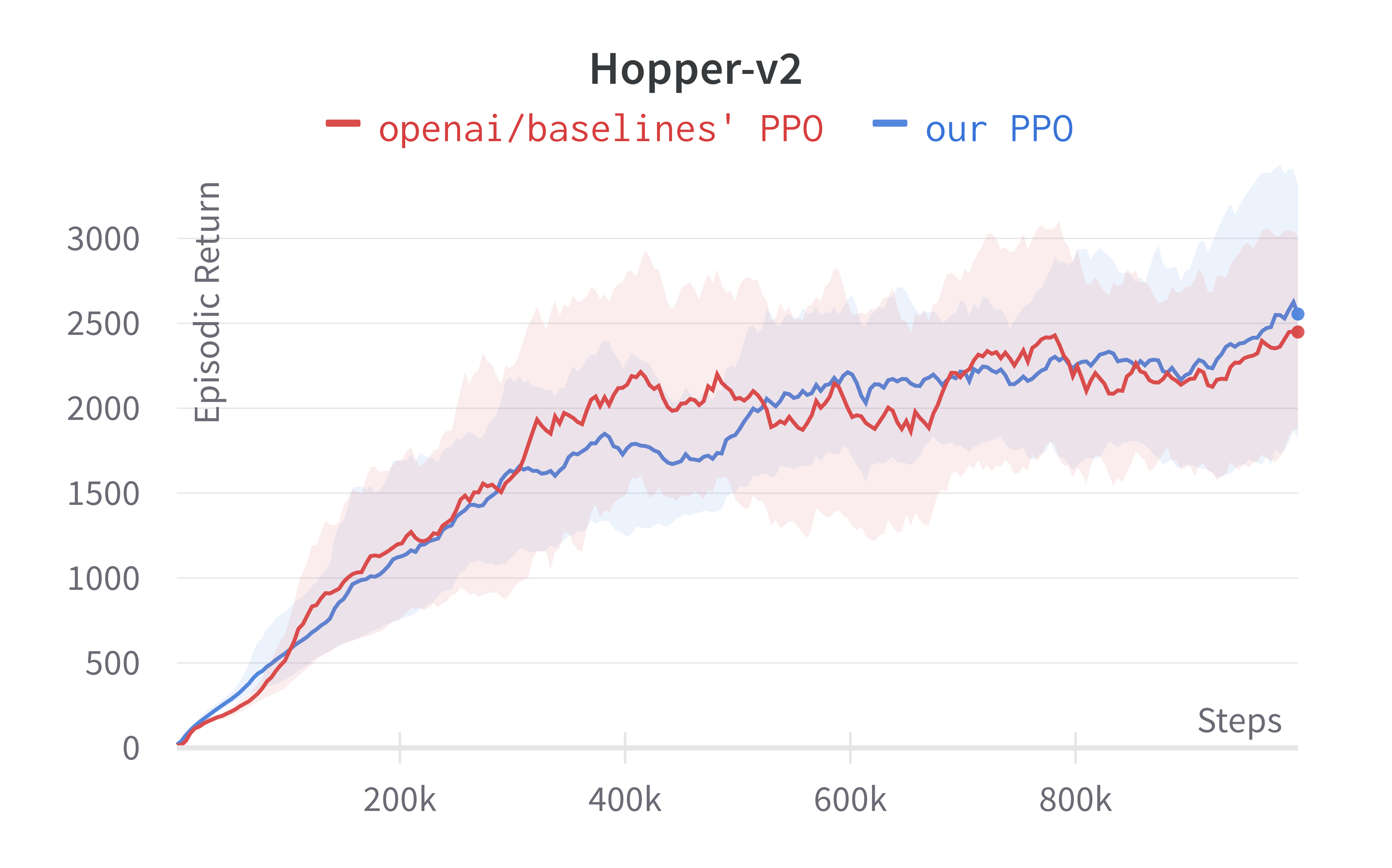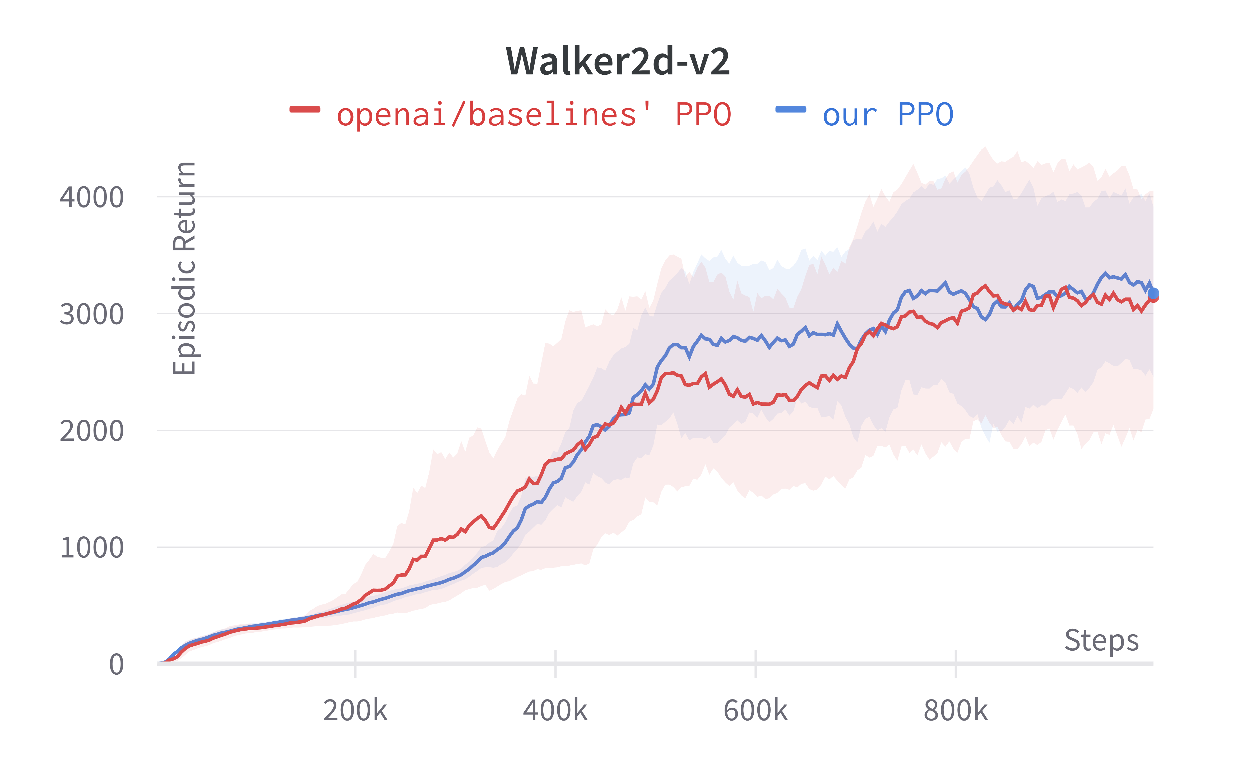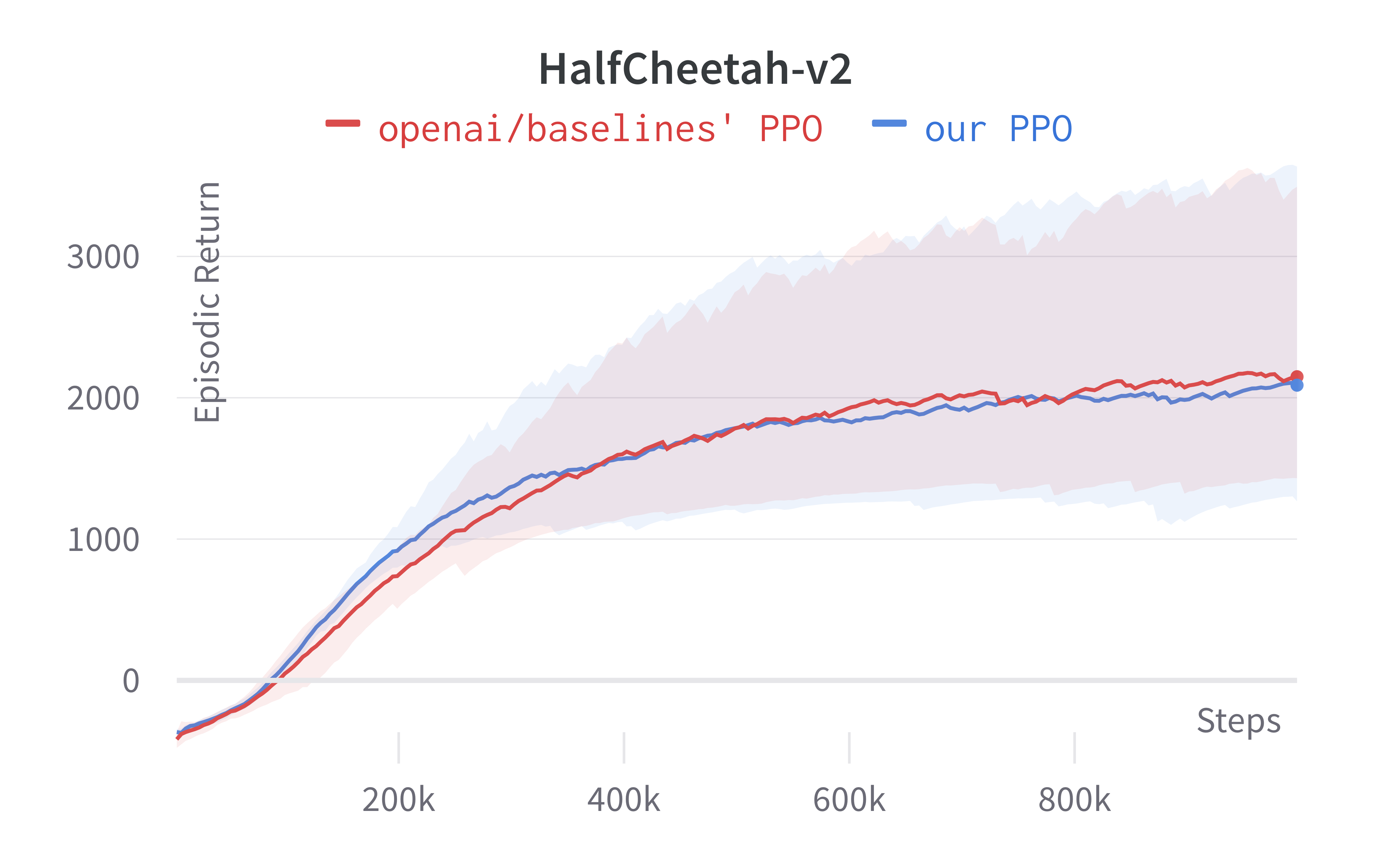
|
||
|
||
> Tracked MuJoCo experiments (click to show the interactive panel)
|
||
|
||
## 5 LSTM implementation details
|
||
|
||
Next, we introduce the 5 details for implementing LSTM.
|
||
|
||
1. Layer initialization for LSTM layers ([a2c/utils.py#L84-L86](https://github.com/openai/baselines/blob/ea25b9e8b234e6ee1bca43083f8f3cf974143998/baselines/a2c/utils.py#L84-L86)) Neural Network
|
||
* The LSTM’s layers’ weights are initialized with `std=1` and biases initialized with `0`.
|
||
|
||
2. Initialize the LSTM states to be zeros ([common/models.py#L179](https://github.com/openai/baselines/blob/ea25b9e8b234e6ee1bca43083f8f3cf974143998/baselines/common/models.py#L179)) Neural Network
|
||
* The hidden and cell states of LSTM are initialized with zeros.
|
||
|
||
3. Reset LSTM states at the end of the episode ([common/models.py#L141](https://github.com/openai/baselines/blob/ea25b9e8b234e6ee1bca43083f8f3cf974143998/baselines/common/models.py#L141)) Theory
|
||
* During rollouts or training, an end-of-episode flag is passed to the agent so that it can reset The LSTM states to zeros.
|
||
|
||
4. Prepare sequential rollouts in mini-batches ([a2c/utils.py#L81](https://github.com/openai/baselines/blob/ea25b9e8b234e6ee1bca43083f8f3cf974143998/baselines/a2c/utils.py#L81)) Theory
|
||
* Under the non-LSTM setting, the mini-batches fetch randomly-indexed training data because the ordering of the training data doesn’t matter. However, the ordering of the training data does matter in the LSTM setting. As a result, the mini-batches fetch the sequential training data from sub-environments.
|
||
|
||
5. Reconstruct LSTM states during training ([a2c/utils.py#L81](https://github.com/openai/baselines/blob/ea25b9e8b234e6ee1bca43083f8f3cf974143998/baselines/a2c/utils.py#L81)) Theory
|
||
* The algorithm saves a copy of the LSTM states `initial_lstm_state` before rollouts. During training, the agent then sequentially reconstruct the LSTM states based on the `initial_lstm_state`. This process ensures that we reconstructed the probability distributions used in rollouts.
|
||
|
||
We make [~60 lines of code](https://www.diffchecker.com/RelaUQdN) change to `ppo_atari.py` to incorporate these 5 details, resulting in a self-contained `ppo_atari_lstm.py` ([link](https://github.com/vwxyzjn/ppo-implementation-details/blob/main/ppo_atari_lstm.py)) that has 385 lines of code. The following shows the file difference between the `ppo_atari.py` (left) and `ppo_atari_lstm.py` (right).
|
||
|
||
To run the experiments, we use the Atari hyperparameters again and remove the frame stack (i.e., setting the number of frames stacked to 1). Below are the benchmarked results.
|
||
|
||

|
||
|
||
> Tracked Atari LSTM experiments (click to show the interactive panel)
|
||
|
||
## 1 `MultiDiscrete` action space detail
|
||
|
||
The `MultiDiscrete` space is often useful to describe action space for more complicated games. The Gym’s official documentation explains `MultiDiscrete` action space as follows:
|
||
|
||
```
|
||
# https://github.com/openai/gym/blob/2af816241e4d7f41a000f6144f22e12c8231a112/gym/spaces/multi_discrete.py#L8-L25
|
||
class MultiDiscrete(Space):
|
||
"""
|
||
- The multi-discrete action space consists of a series of discrete action spaces with different number of actions in each
|
||
- It is useful to represent game controllers or keyboards where each key can be represented as a discrete action space
|
||
- It is parametrized by passing an array of positive integers specifying number of actions for each discrete action space
|
||
Note: Some environment wrappers assume a value of 0 always represents the NOOP action.
|
||
e.g. Nintendo Game Controller
|
||
- Can be conceptualized as 3 discrete action spaces:
|
||
1) Arrow Keys: Discrete 5 - NOOP[0], UP[1], RIGHT[2], DOWN[3], LEFT[4] - params: min: 0, max: 4
|
||
2) Button A: Discrete 2 - NOOP[0], Pressed[1] - params: min: 0, max: 1
|
||
3) Button B: Discrete 2 - NOOP[0], Pressed[1] - params: min: 0, max: 1
|
||
- Can be initialized as
|
||
MultiDiscrete([ 5, 2, 2 ])
|
||
"""
|
||
...
|
||
```
|
||
|
||
Next, we introduce 1 detail for handling `MultiDiscrete` action space:
|
||
|
||
1. Independent action components ([common/distributions.py#L215-L220](https://github.com/openai/baselines/blob/9b68103b737ac46bc201dfb3121cfa5df2127e53/baselines/common/distributions.py#L215-L220)Theory
|
||
* In `MultiDiscrete` action spaces, the actions are represented with multiple discrete values. For example, the action of $a_{t} = \left[\right. a_{t}^{1} , a_{t}^{2} \left]\right. = \left[\right. 0 , 1 \left]\right.$ might mean to press the up arrow key and press button A. To account for this difference, PPO treats $\left[\right. a_{t}^{1} , a_{t}^{2} \left]\right.$ as probabilistically independent action components, therefore calculating $p r o b \left(\right. a_{t} \left.\right) = p r o b \left(\right. a_{t}^{1} \left.\right) \cdot p r o b \left(\right. a_{t}^{2} \left.\right)$.
|
||
* AlphaStar ([Vinyals et al., 2019](https://iclr-blog-track.github.io/2022/03/25/ppo-implementation-details/#Vinyals2019)) and OpenAI Five ([Berner et al., 2019](https://iclr-blog-track.github.io/2022/03/25/ppo-implementation-details/#Berner2019)) adopts the `MultiDiscrete` action spaces. For example, OpenAI Five’s action space is essentially `MultiDiscrete([ 30, 4, 189, 81 ])`, as shown by the following quote:
|
||
> All together this produces a combined factorized action space size of up to 30 × 4 × 189 × 81 = 1, 837, 080 dimensions
|
||
|
||
We make [~36 lines of code](https://www.diffchecker.com/8fsnhwUI) change to `ppo_atari.py` to incorporate this 1 detail, resulting in a self-contained `ppo_multidiscrete.py` ([link](https://github.com/vwxyzjn/ppo-implementation-details/blob/main/ppo_multidiscrete.py)) that has 335 lines of code. The following shows the file difference between the `ppo_atari.py` (left) and `ppo_multidiscrete.py` (right).
|
||
|
||
To run the experiments, we use the Atari hyperparameters again and use Gym-μRTS ([Huang et al, 2021](https://iclr-blog-track.github.io/2022/03/25/ppo-implementation-details/#Huang2021)) as the simulation environment.
|
||
|
||
```
|
||
def gym_microrts():
|
||
return dict(
|
||
nsteps=128, nminibatches=4,
|
||
lam=0.95, gamma=0.99, noptepochs=4, log_interval=1,
|
||
ent_coef=.01,
|
||
lr=lambda f : f * 2.5e-4,
|
||
cliprange=0.1,
|
||
)
|
||
```
|
||
|
||
Below are the benchmarked results.
|
||
|
||

|
||
|
||
> Tracked Gym-MicroRTS experiments (click to show the interactive panel)
|
||
|
||
## 4 Auxiliary implementation details
|
||
|
||
Next, we introduce 4 auxiliary techniques that are not used (by default) in the official PPO implementations but are potentially useful in special situations.
|
||
|
||
1. Clip Range Annealing ([ppo2/ppo2.py#L137](https://github.com/openai/baselines/blob/ea25b9e8b234e6ee1bca43083f8f3cf974143998/baselines/ppo2/ppo2.py#L137)) Code-level Optimizations
|
||
* The clip coefficient of PPO can be annealed similar to how the learning rate is annealed. However, the clip range annealing is actually used by default.
|
||
|
||
2. Parallellized Gradient Update ([ppo2/model.py#L131](https://github.com/openai/baselines/blob/ea25b9e8b234e6ee1bca43083f8f3cf974143998/baselines/ppo2/model.py#L131)) Code-level Optimizations
|
||
* The policy gradient is calculated in parallel using multiple processes, mainly used in `ppo1` and not used by default in `ppo2`. Such as paradigm could improve training time by making use of all the available processes.
|
||
|
||
3. Early Stopping of the policy optimizations ([ppo/ppo.py#L269-L271](https://github.com/openai/spinningup/blob/038665d62d569055401d91856abb287263096178/spinup/algos/pytorch/ppo/ppo.py#L269-L271)) Code-level Optimizations
|
||
* This is not actually an implementation detail of _openai/baselines_, but rather an implementation detail in John Schulman’s [modular_rl](https://github.com/joschu/modular_rl/blob/5481b117aa30d3eb8e9ad79abce06378d60dcd45/modular_rl/ppo.py#L48) and _openai/spinningup_ ([TF 1.x](https://github.com/openai/spinningup/blob/038665d62d569055401d91856abb287263096178/spinup/algos/tf1/ppo/ppo.py#L234), [Pytorch](https://github.com/openai/spinningup/blob/038665d62d569055401d91856abb287263096178/spinup/algos/pytorch/ppo/ppo.py#L269-L271)). It can be considered as an additional mechanism to explicitly enforce the trust-region constraint, on top of the fixed hyperparameter `noptepochs` proposed in the original implementation by [Schulman et al. (2017)](https://iclr-blog-track.github.io/2022/03/25/ppo-implementation-details/#Schulman2017).
|
||
* More specifically, it starts by tracking an approximate average KL divergence between the policy before and after one update step to its network weights. In case said KL divergence exceeds a preset threshold, the updates to the policy weights are preemptively stopped. [Dossa et al.](https://iclr-blog-track.github.io/2022/03/25/ppo-implementation-details/#Dossa2021) suggest that early stopping can serve as an alternative method to tune the number of update epochs. We also included this early stopping method in our implementation [(via `--target-kl 0.01`)](https://github.com/vwxyzjn/ppo-implementation-details/blob/eb40cbe172309dcda24a8e93a32269d819e5513d/ppo.py#L71), but toggled it off by default.
|
||
* Note, however, that while _openai/spinningup_ only early stops the updates to the policy, our implementation early stops both the policy and the value network updates.
|
||
|
||
4. Invalid Action Masking ([Vinyals et al., 2017](https://iclr-blog-track.github.io/2022/03/25/ppo-implementation-details/#Vinyals2017); [Huang and Ontañón, 2020](https://iclr-blog-track.github.io/2022/03/25/ppo-implementation-details/#HuangOntanon2020)) Theory
|
||
* Invalid action masking is a technique employed most prominently in AlphaStar ([Vinyals et al., 2019](https://iclr-blog-track.github.io/2022/03/25/ppo-implementation-details/#Vinyals2019)) and OpenAI Five ([Berner et al., 2019](https://iclr-blog-track.github.io/2022/03/25/ppo-implementation-details/#Berner2019)) to avoid executing invalid actions in a given game state when the agents are being trained using policy gradient algorithms. Specifically, invalid action masking is implemented by replacing the logits corresponding to the invalid actions with negative infinity before passing the logits to softmax. [Huang and Ontañón, 2020](https://iclr-blog-track.github.io/2022/03/25/ppo-implementation-details/#HuangOntanon2020) show such a paradigm **actually makes the gradients corresponding to invalid actions zeros**. Furthermore, [Huang et al, 2021](https://iclr-blog-track.github.io/2022/03/25/ppo-implementation-details/#Huang2021) demonstrated invalid action masking to be the critical technique in training agents to win against all past μRTS bots they tested.
|
||
|
||
Notably, we highlight the effect of invalid action masking. We make [~30 lines of code](https://www.diffchecker.com/wBUb6Zne) change to `ppo_multidiscrete.py` to incorporate invalid action masking, resulting in a self-contained `ppo_multidiscrete_mask.py` ([link](https://github.com/vwxyzjn/ppo-implementation-details/blob/main/ppo_multidiscrete_mask.py)) that has 363 lines of code. The following shows the file difference between the `ppo_multidiscrete.py` (left) and `ppo_multidiscrete_mask.py` (right).
|
||
|
||
To run the experiments, we use the Atari hyperparameters again and use an older version of Gym-μRTS ([Huang et al, 2021](https://iclr-blog-track.github.io/2022/03/25/ppo-implementation-details/#Huang2021)) as the simulation environment. Below are the benchmarked results.
|
||
|
||
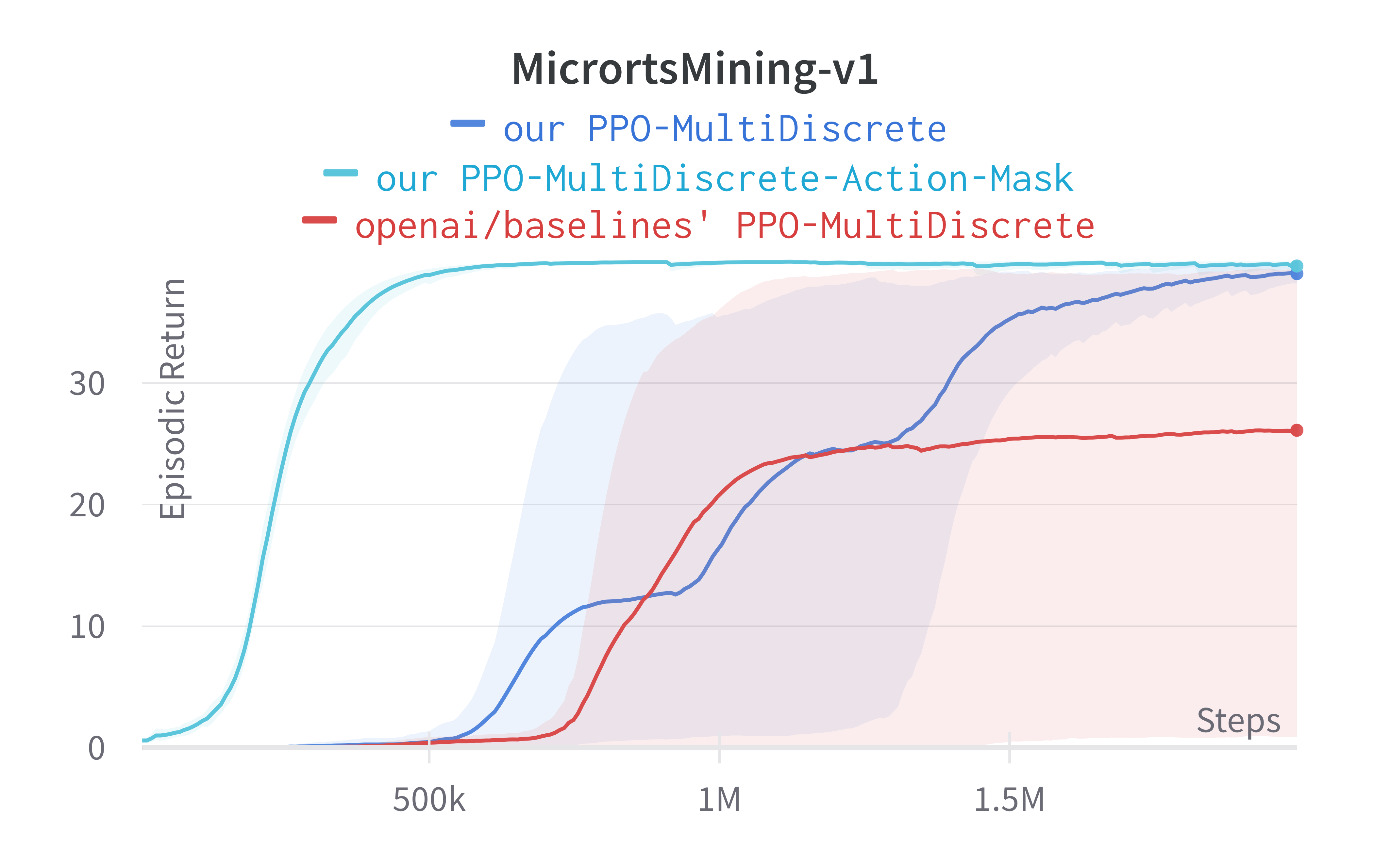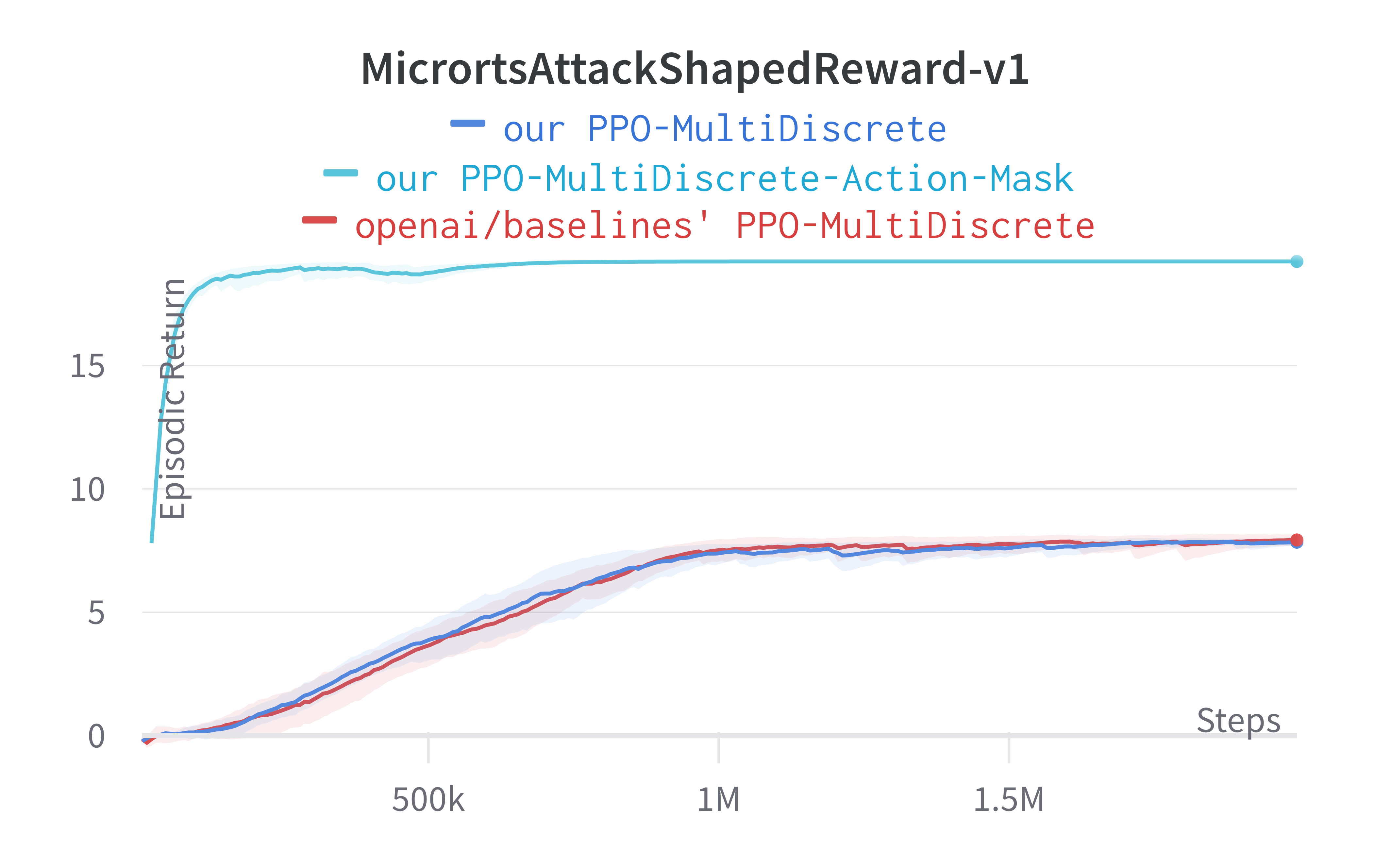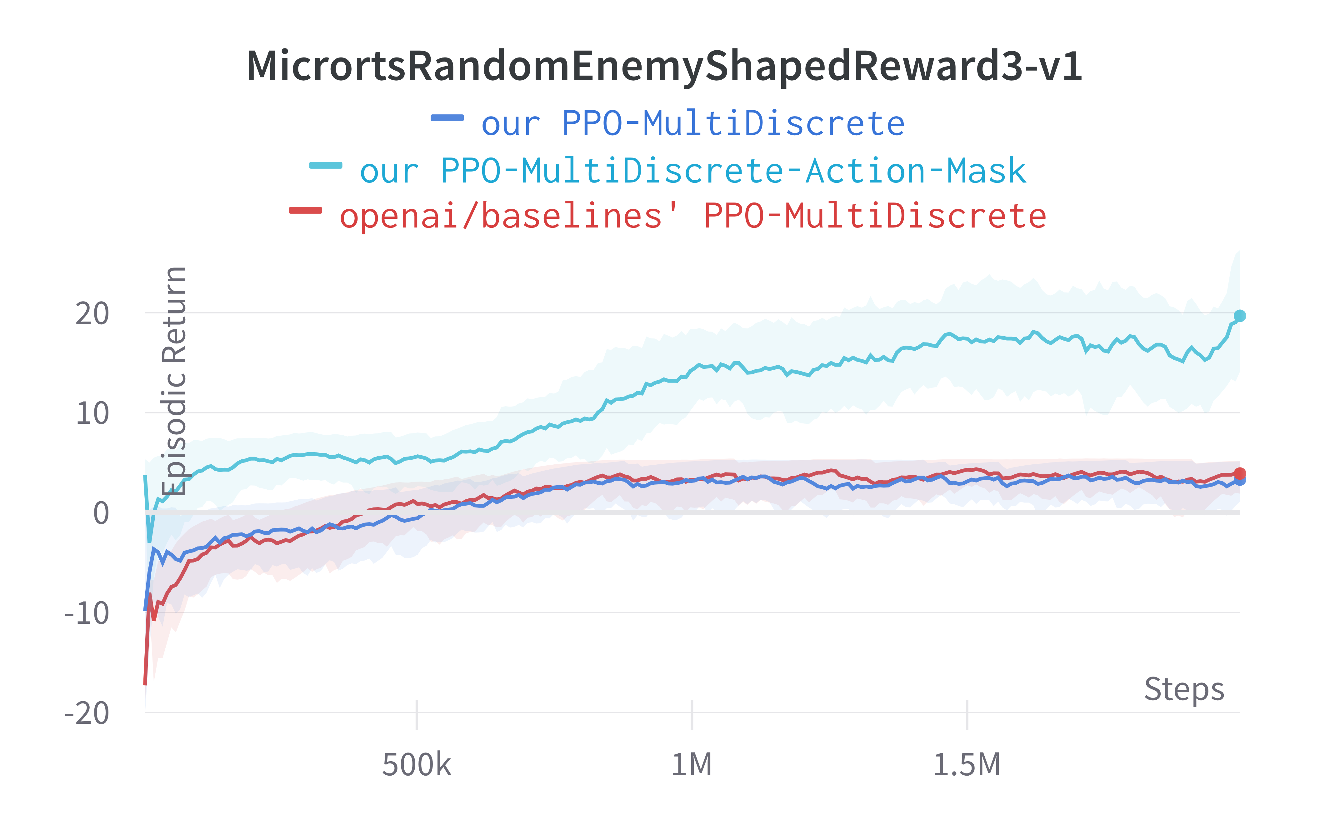
|
||
|
||
> Tracked Gym-MicroRTS + Action Mask experiments (click to show the interactive panel)
|
||
|
||
## Results
|
||
|
||
As shown under each section, our implementations match the results of the original implementation closely. This close matching also extends to other metrics such as policy and value losses. We have made an interactive HTML below for interested viewers to compare other metrics:
|
||
|
||
## Recommendations
|
||
|
||
During our reproduction, we have found a number of useful debugging techniques. They are as follows:
|
||
|
||
1. **Seed everything**: One debugging approach is to seed everything and then observe when things start to differ from the reference implementation. So you could use the same seed for your implementation and mine, check if the observation returned by the environment is the same, then check if the sample the actions are the same. By following the steps, you would check everything to make sure they are aligned (e.g. print out `values.sum()` see if yours match the reference implementation). In the past, we have done this with the [pytorch-a2c-ppo-acktr-gail](https://github.com/ikostrikov/pytorch-a2c-ppo-acktr-gail) repository and ultimately figured out a bug with our implementation.
|
||
2. **Check if `ratio=1`**: Check if the `ratio` are always 1s during the first epoch and first mini-batch update, when new and old policies are the same and therefore the `ratio` are 1s and has nothing to clip. If `ratio` are not 1s, it means there is a bug and the program has not reconstructed the probability distributions used in rollouts.
|
||
3. **Check Kullback-Leibler (KL) divergence**: It is often useful to check if KL divergence goes too high. We have generally found the `approx_kl` stays below 0.02, and if `approx_kl` becomes too high it usually means the policy is changing too quickly and there is a bug.
|
||
4. **Check other metrics**: As shown in the Results section, the other metrics such as policy and value losses in our implementation also closely match those in the original implementation. So if your policy loss’ curve looks very different than the reference implementation, there might be a bug.
|
||
5. **Rule of thumb: 400 episodic return in breakout**: Check if your PPO could obtain 400 episodic return in breakout. We have found this to be a practical rule of thumb to determine the fidelity of online PPO implementations in GitHub. Often we found PPO repositories not able to do this, and we know they probably do not match all implementation details of `openai/baselines`’ PPO.
|
||
|
||
If you are doing research using PPO, consider adopting the following recommendations to help improve the reproducibility of your work:
|
||
|
||
1. **Enumerate implementation details used**: If you have implemented PPO as the baseline for your experiment, you should specify which implementation details you are using. Consider using bullet points to enumerate them like done in this blog post.
|
||
2. **Release locked source code**: Always open source your code whenever possible and make sure the code runs. We suggest adopting proper dependency managers such as [poetry](https://python-poetry.org/) or [pipenv](https://pipenv.pypa.io/en/latest/) to lock your dependencies. In the past, we have encountered numerous projects that are based on `pip install -e .`, which 80% of the time would fail to run due to some obscure errors. Having a pre-built `docker` image with all dependencies installed can also help in case the dependencies packages are not hosted by package managers after deprecation.
|
||
3. **Track experiments**: Consider using an experiment management software to track your metrics, hyperparameters, code, and others. They can boost your productivity by saving hundreds of hours spent on `matplotlib` and worrying about how to display data. Commercial solutions (usually more mature) include [Weights and Biases](https://wandb.ai/) and [Neptune](https://neptune.ai/), and open-source solutions include [Aim](https://github.com/aimhubio/aim), [ClearML](https://github.com/allegroai/clearml), [Polyaxon](https://github.com/polyaxon/polyaxon).
|
||
4. **Adopt single-file implementation**: If your research requires more tweaking, consider implementing your algorithms using single-file implementations. This blog does this and creates standalone files for different environments. For example, our `ppo_atari.py` contains all relevant code to handle Atari games. Such a paradigm has the following benefits at the cost of duplicate and harder-to-refactor code:
|
||
* _Easier to see the whole picture_: Because each file is self-contained, people can easily spot all relevant implementation details of the algorithm. Such a paradigm also reduces the burden to understand how files like `env.py`, `agent.py`, `network.py` work together like in typical RL libraries.
|
||
* _Faster developing experience_: Usually, each file like `ppo.py` has significantly less LOC compared to RL libraries’ PPO. As a result, it’s often easier to prototype new features without having to do subclassing and refactoring.
|
||
* _Painless performance attribution_: If a new version of our algorithm has obtained higher performance, we know this single file is exactly responsible for the performance improvement. To attribute the performance improvement, we can simply do a `filediff` between the current and past versions, and every line of code change is made explicit to us.
|
||
|
||
## Discussions
|
||
|
||
## Does modularity help RL libraries?
|
||
|
||
This blog post demonstrates reproducing PPO is a non-trivial effort, even though PPO’s source code is readily available for reference. Why is it the case? We think one important reason might be that **modularity disperses implementation details**.
|
||
|
||
Almost all RL libraries have adopted modular design, featuring different modules / files like `env.py`, `agent.py`, `network.py`, `utils.py`, `runner.py`, etc. The nature of modularity necessarily puts implementation details into different files, which is usually great from a software engineering perspective. That is, we don’t have to know how other components work when we just work on `env.py`. Being able to treat other components as black boxes has empowered us to work on large and complicated systems for the last decades.
|
||
|
||
However, this practice might clash hard with ML / RL: as the library grows, it becomes harder and harder to grasp all implementation details w.r.t an algorithm, whereas recognizing all implementation details has become increasingly important, as indicated by this blog post, [Engstrom, Ilyas, et al., 2020](https://iclr-blog-track.github.io/2022/03/25/ppo-implementation-details/#Engstrom), and [Andrychowicz, et al., 2021](https://iclr-blog-track.github.io/2022/03/25/ppo-implementation-details/#Andrychowicz). So what can we do?
|
||
|
||
Modular design still offers numerous benefits such as 1) easy-to-use interface, 2) integrated test cases, 3) easy to plug different components and others. To this end, good RL libraries are valuable, and we recommend them to write good documentation and refactor libraries to adopt new features. For algorithmic researchers, however, we recommend considering single-file implementations because they are straightforward to read and extend.
|
||
|
||
## Is asynchronous PPO better?
|
||
|
||
Not necessarily. The high-throughput variant Asynchronous PPO (APPO) ([Berner et al., 2019](https://iclr-blog-track.github.io/2022/03/25/ppo-implementation-details/#Berner2019)) has obtained more attention in recent years. APPO eliminates the idle time in the original PPO implementation (e.g., have to wait for all $N$ environments to return observations), resulting in much higher throughput, GPU and CPU utilization. However, APPO involves performance-reducing side-effects, namely stale experiences ([Espeholt et al., 2018](https://iclr-blog-track.github.io/2022/03/25/ppo-implementation-details/#IMPALA)), and we have found insufficient evidence to ascertain its improvement. The biggest issue is:
|
||
|
||
**Underbenchmarked APPO implementation**: RLlib has an [APPO implementation](https://docs.ray.io/en/latest/rllib-algorithms.html#appo), yet its documentation contains no benchmark information and suggest “APPO is not always more efficient; it is often better to use standard PPO or IMPALA.” Sample Factory ([Petrenko et al, 2020](https://iclr-blog-track.github.io/2022/03/25/ppo-implementation-details/#Petrenko)) presents more benchmark results, but its support for Atari games is still a [work in progress](https://github.com/alex-petrenko/sample-factory/issues/51). To our knowledge, there is no APPO implementation that simultaneously works with Atari games, MuJoCo or Pybullet tasks, MultiDiscrete action spaces and with an LSTM.
|
||
|
||
While APPO is intuitively valuable for CPU-intensive tasks such as Dota 2, this blog post recommends an alternative approach to speed up PPO: **make the vectorized environments really fast**. Initially, the vectorized environments are implemented in python, which is slow. More recently, researchers have proposed to use accelerated vectorized environments. For example,
|
||
|
||
1. Procgen [(Cobbe et al, 2020)](https://iclr-blog-track.github.io/2022/03/25/ppo-implementation-details/#Cobbe) uses C++ to implement native vectorized environments, resulting in much higher throughput when setting $N = 64$ ($N$ is the number of environments),
|
||
2. [Envpool](https://github.com/sail-sg/envpool) uses C++ to offer native vectorized environments for Atari and classic control games,
|
||
3. Nvidia’s [Isaac Gym](https://developer.nvidia.com/isaac-gym)[(Makoviychuk et al., 2021)](https://iclr-blog-track.github.io/2022/03/25/ppo-implementation-details/#Makoviychuk) uses `torch` to write hardware-accelerated vectorized environments, allowing the users to spin up $N = 4096$ environments easily,
|
||
4. Google’s [Brax](https://github.com/google/brax) uses jax to write hardware-accelerated vectorized environments, allowing the users to spin up $N = 2048$ environments easily and solve robotics tasks like `Ant` in minutes compared to hours of training in MuJoCo.
|
||
|
||
In the following section, we demonstrate accelerated training with PPO + envpool in the Atari game Pong.
|
||
|
||
### Solving Pong in 5 minutes with PPO + Envpool
|
||
|
||
[Envpool](https://github.com/sail-sg/envpool) is a recent work that offers accelerated vectorized environments for Atari by leveraging C++ and thread pools. Our PPO gets a free and side-effects-free performance boost by simply adopting it. We make [~60 lines of code](https://www.diffchecker.com/RafLuYD6) change to `ppo_atari.py` to incorporate this 1 detail, resulting in a self-contained `ppo_atari_envpool.py` ([link](https://github.com/vwxyzjn/ppo-implementation-details/blob/main/ppo_atari_envpool.py)) that has 365 lines of code. The following shows the file difference between the `ppo_atari.py` (left) and `ppo_atari_envpool.py` (right).
|
||
|
||
As shown below, Envpool + PPO runs 3x faster without side effects (as in no loss of sample efficiency):
|
||
|
||
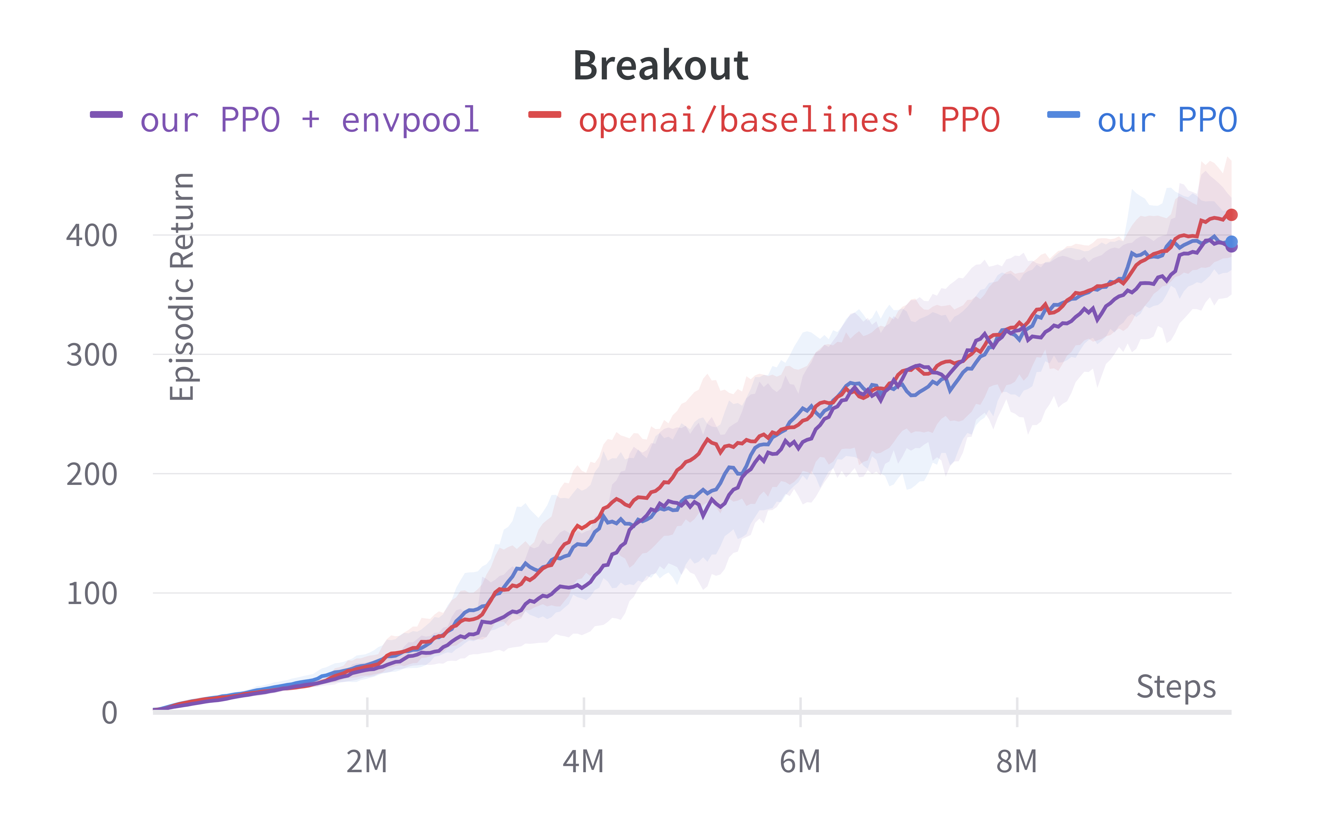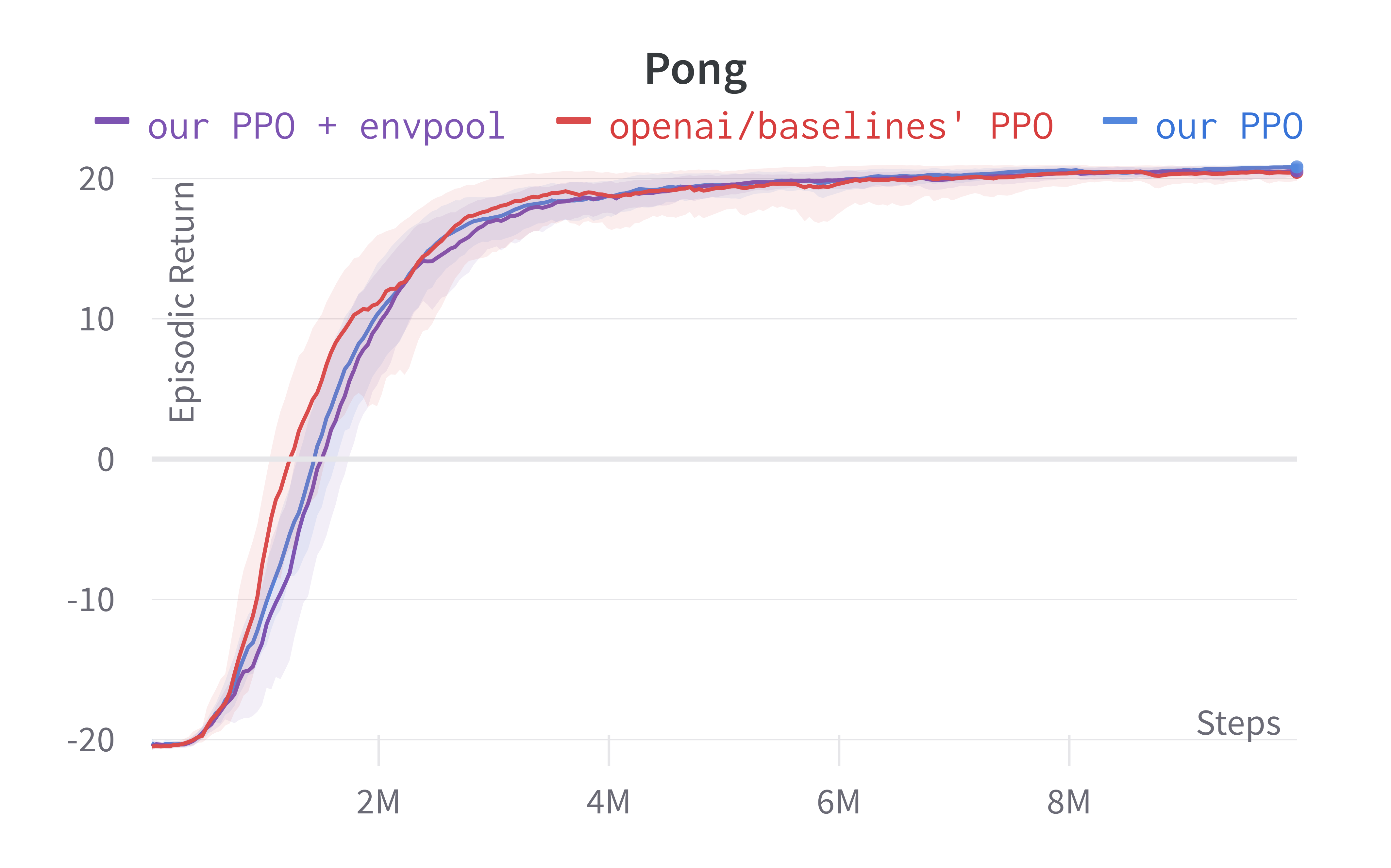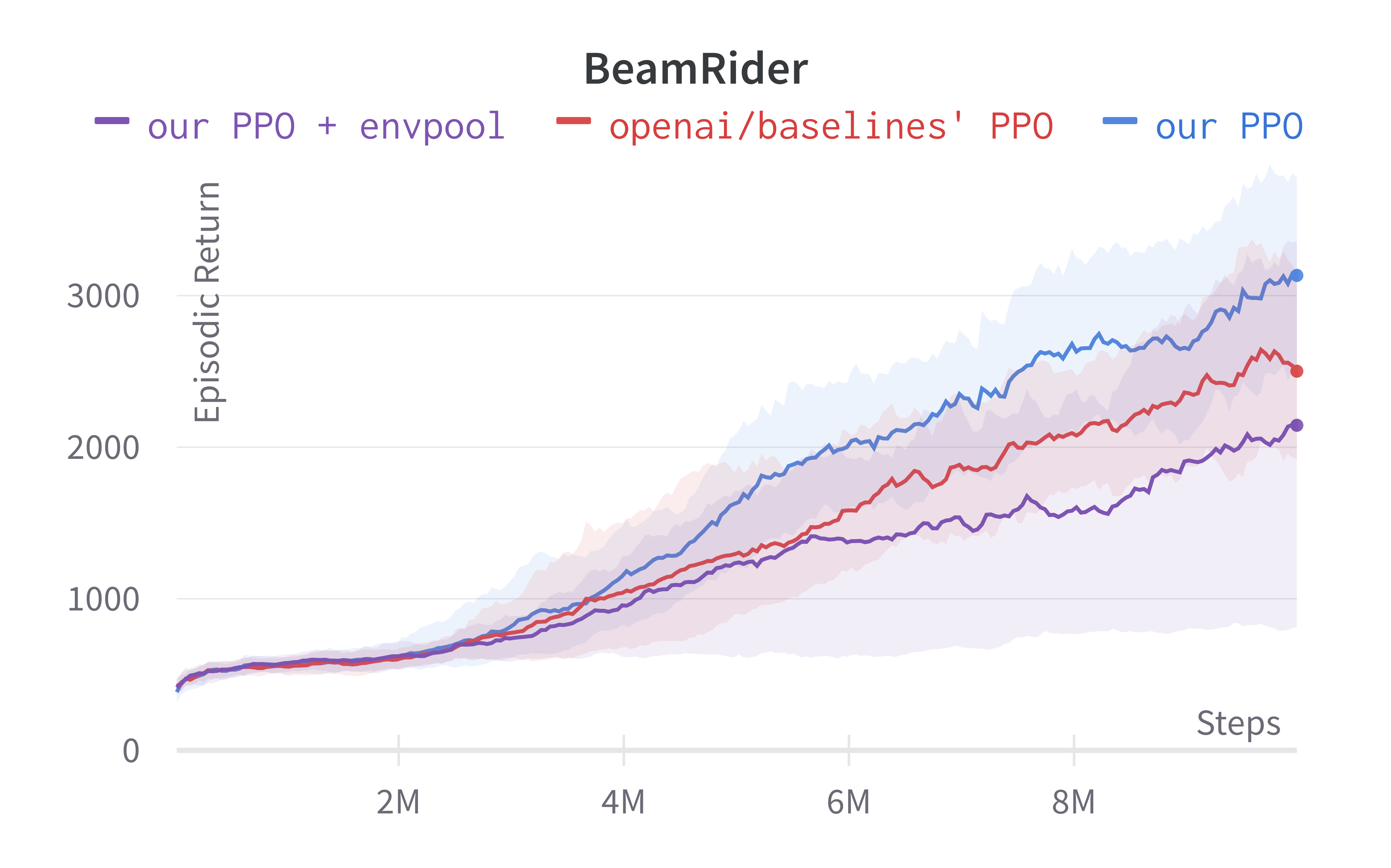
|
||
|
||
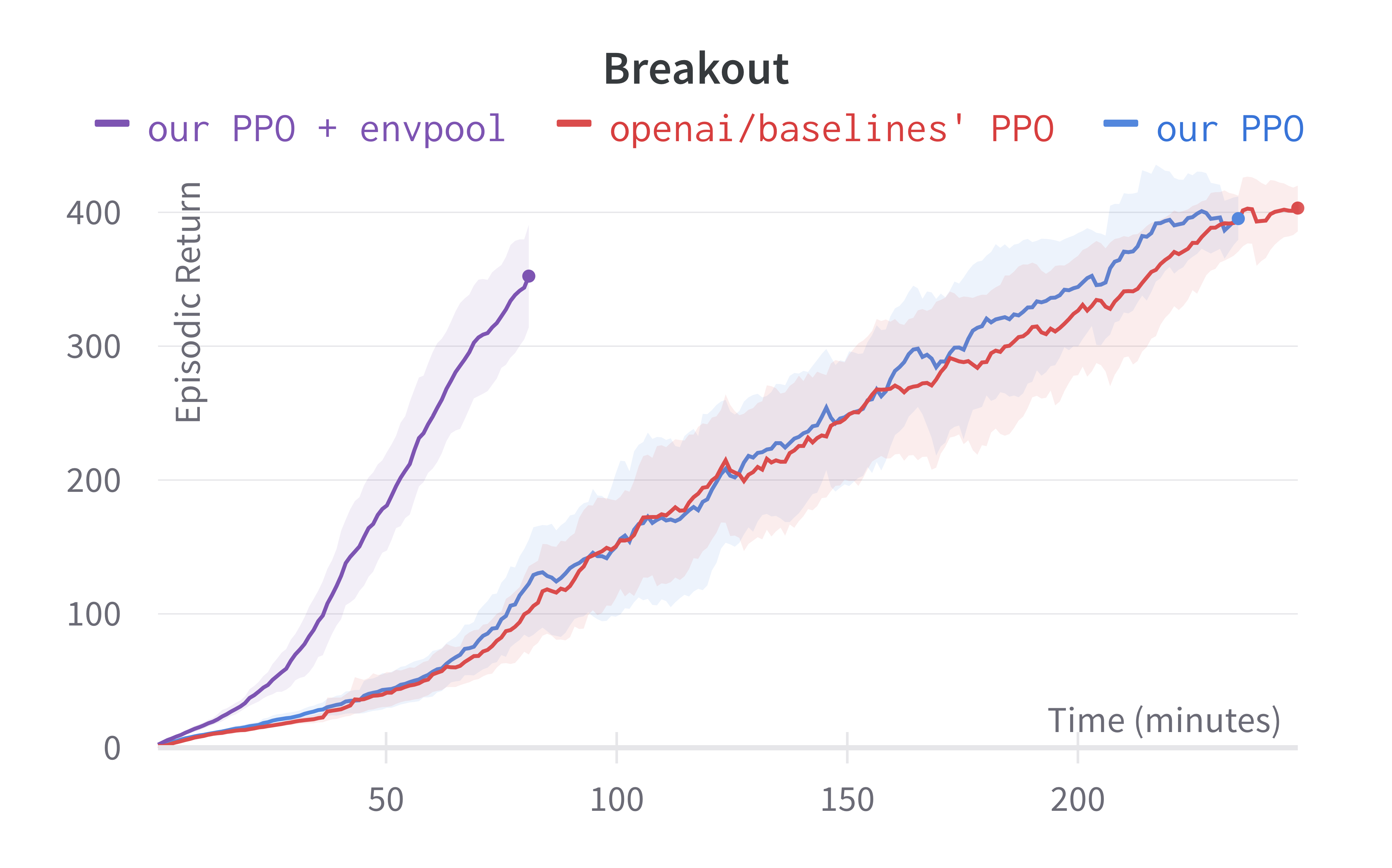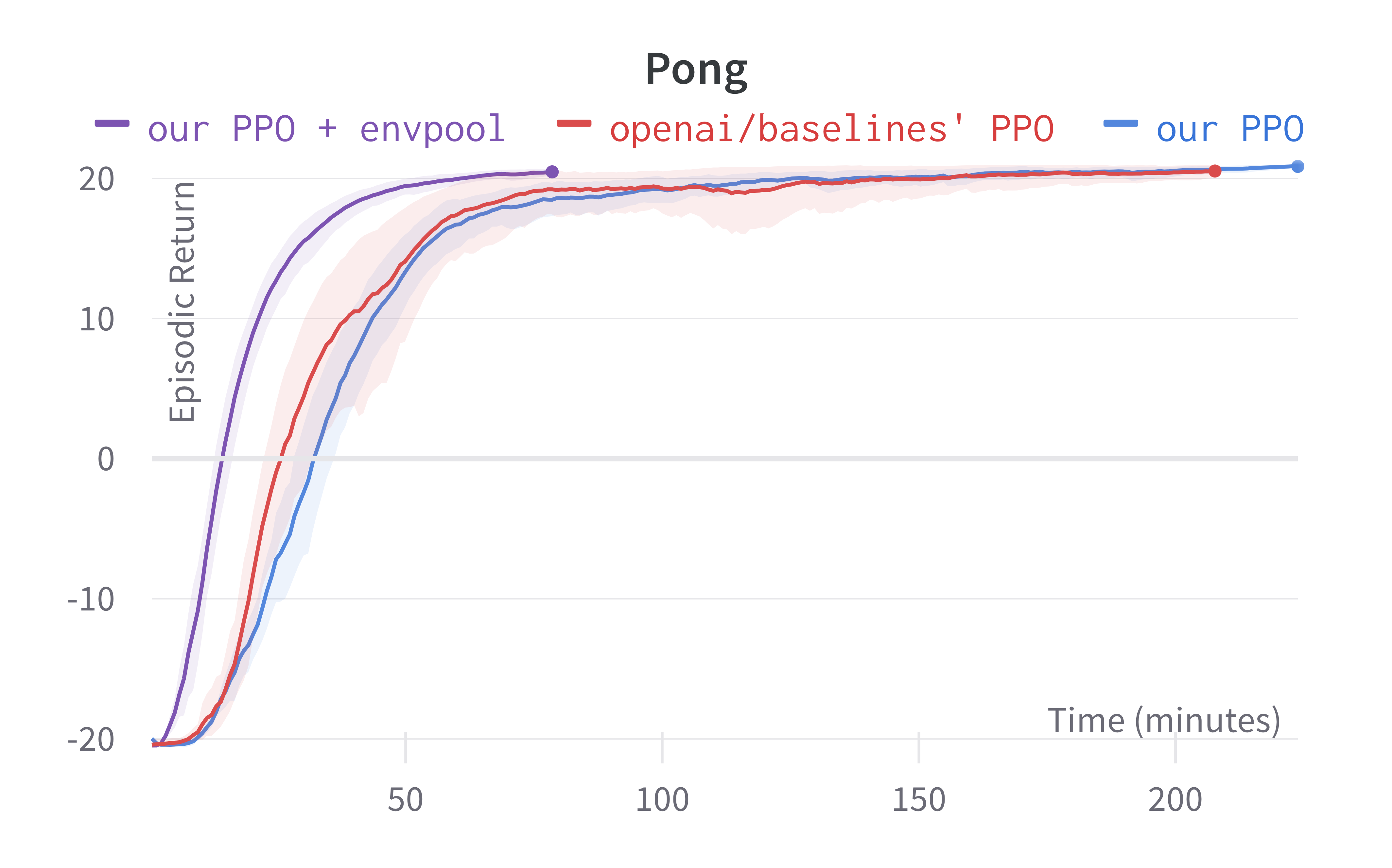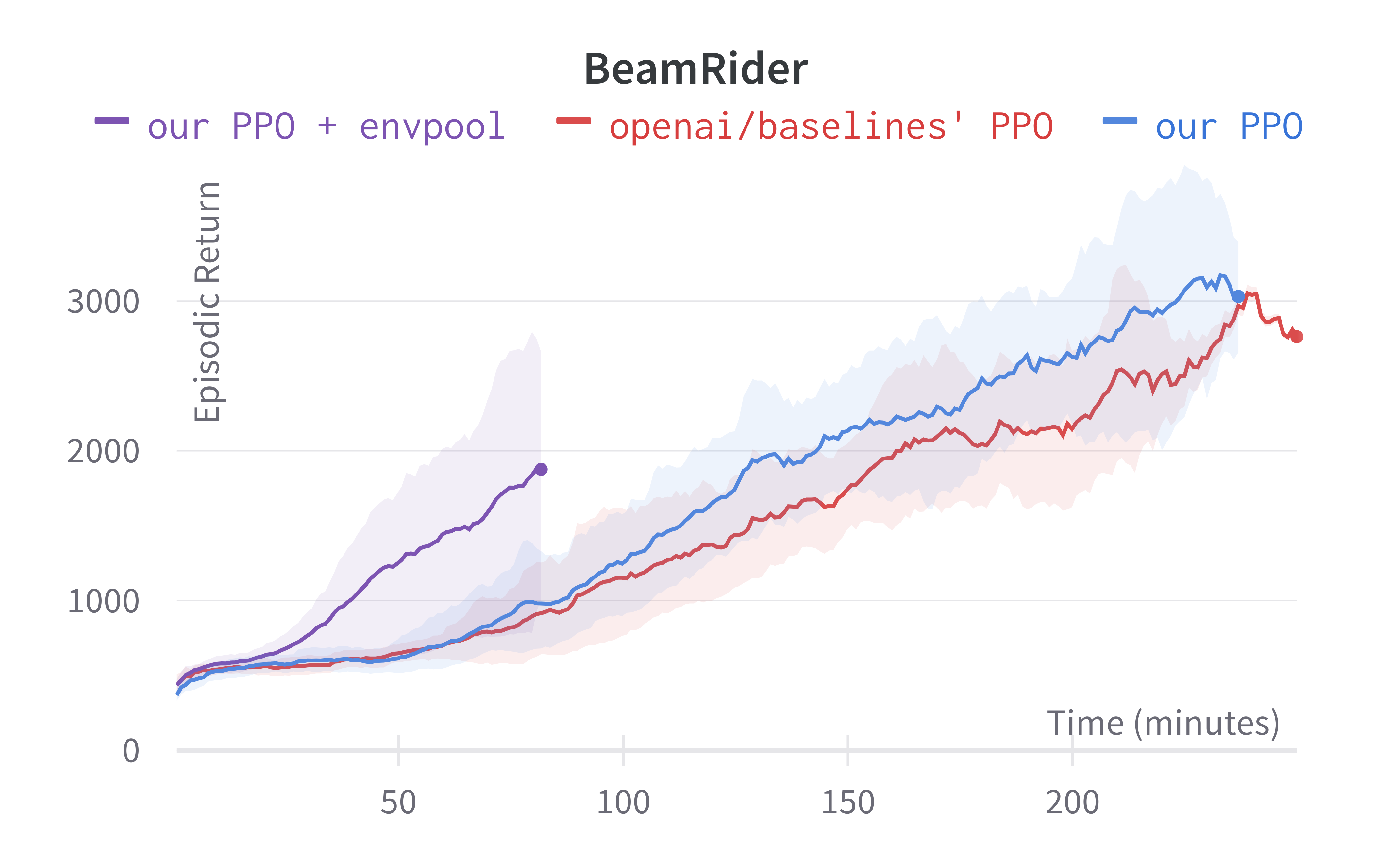
|
||
|
||
> Tracked Atari + Envpool experiments (click to show the interactive panel)
|
||
|
||
Two quick notes: 1) the performance deterioration in BeamRider is largely due to a degenerate random seed, and 2) Envpool uses the v5 ALE environments but has processed them the same way as the v4 ALE environments used in our previous experiments. Furthermore, by tuning the hyperparameters, we obtained a run that solves Pong in 5 mins. This performance is even comparable to IMPALA’s ([Espeholt et al., 2018](https://iclr-blog-track.github.io/2022/03/25/ppo-implementation-details/#IMPALA)) results:
|
||
|
||
We think this raises a practical consideration: adopting async RL such as IMPALA could be more difficult than just making your vectorized environments fast.
|
||
|
||
## Request for Research
|
||
|
||
Given this blog post, we believe the community understands PPO better and would be in a much better place to make improvements. Here are a few suggested areas for research.
|
||
|
||
1. **Alternative choices**: As we have walked through the different details of PPO, it seems that some of them result from arbitrary choices. It would be interesting to investigate alternative choices and see how such change affects results. You can find below a non-exhaustive list of tracks to explore:
|
||
* use of a different Atari pre-processing (as partially explored by [Machado et al., 2018)](https://iclr-blog-track.github.io/2022/03/25/ppo-implementation-details/#Machado2018))
|
||
* use of a different distribution for continuous actions ([Beta distribution](http://proceedings.mlr.press/v70/chou17a/chou17a.pdf), squashed Gaussian, Gaussian with full covariance, …), it will most probably require some tuning
|
||
* use of a state-dependent standard deviation when using continuous actions (with or without backpropagation of the gradient to the whole actor network)
|
||
* use of a different initialization for LSTM (ones instead of zeros, random noise, learnable parameter, …), use of GRU cells instead of LSTM
|
||
|
||
2. **Vectorized architecture for experience-replay-based methods**: Experience-replay-based methods such as DQN, DDPG, and SAC are less popular than PPO due to a few reasons: 1) they generally have lower throughput due to a single simulation environment (also means lower GPU utilization), and 2) they usually have higher memory requirement (e.g., DQN requires the notorious 1M sample replay buffer which could take 32GB memory). Can we apply the vectorized architecture to experience-replay-based methods? The vectorized environments intuitively should replace replay buffer because the environments could also provide uncorrelated experience.
|
||
3. **Value function optimization**: In Phasic Policy Gradient ([Cobbe et al., 2021](https://iclr-blog-track.github.io/2022/03/25/ppo-implementation-details/#Cobbe2021)), optimizing value functions separately turns out to be important. In DQN, the prioritized experience replay significantly boosts performance. Can we apply prioritized experience replay to PPO or just on PPO’s value function?
|
||
|
||
## Conclusion
|
||
|
||
Reproducing PPO’s results has been difficult in the past few years. While recent works conducted ablation studies to provide insight on the implementation details, these works are not structured as tutorials and only focus on details concerning robotics tasks. As a result, reproducing PPO from scratch can become a daunting experience. Instead of introducing additional improvements or doing further ablation studies, this blog post takes a step back and focuses on delivering a thorough reproduction of PPO in all accounts, as well as aggregating, documenting, and cataloging its most salient implementation details. This blog post also points out software engineering challenges in PPO and further efficiency improvement via the accelerated vectorized environments. With these, we believe this blog post will help people understand PPO faster and better, facilitating customization and research upon this versatile RL algorithm.
|
||
|
||
## Acknowledgment
|
||
|
||
We thank [Weights and Biases](https://wandb.ai/) for providing a free academic license that helps us track the experiments. Shengyi would like to personally thank Angelica Pan, Scott Condron, Ivan Goncharov, Morgan McGuire, Jeremy Salwen, Cayla Sharp, Lavanya Shukla, and Aakarshan Chauhan for supporting him in making the video tutorials.
|
||
|
||
### Bibliography
|
||
|
||
[Schulman J, Wolski F, Dhariwal P, Radford A, Klimov O. Proximal policy optimization algorithms. arXiv preprint arXiv:1707.06347. 2017 Jul 20.](http://arxiv.org/abs/1707.06347)
|
||
|
||
[Schulman, J., Moritz, P., Levine, S., Jordan, M., & Abbeel, P. (2015). High-dimensional continuous control using generalized advantage estimation. arXiv preprint arXiv:1506.02438.](http://arxiv.org/abs/1707.06347)
|
||
|
||
[Engstrom L, Ilyas A, Santurkar S, Tsipras D, Janoos F, Rudolph L, Madry A. Implementation matters in deep policy gradients: A case study on ppo and trpo. International Conference on Learning Representations, 2020](https://openreview.net/forum?id=r1etN1rtPB)
|
||
|
||
[Andrychowicz M, Raichuk A, Stańczyk P, Orsini M, Girgin S, Marinier R, Hussenot L, Geist M, Pietquin O, Michalski M, Gelly S. What matters in on-policy reinforcement learning? a large-scale empirical study. International Conference on Learning Representations, 2021](https://openreview.net/forum?id=nIAxjsniDzg)
|
||
|
||
[Mnih V, Kavukcuoglu K, Silver D, Rusu AA, Veness J, Bellemare MG, Graves A, Riedmiller M, Fidjeland AK, Ostrovski G, Petersen S. Human-level control through deep reinforcement learning. nature. 2015 Feb;518(7540):529-33.](https://www.nature.com/articles/nature14236)
|
||
|
||
[Machado MC, Bellemare MG, Talvitie E, Veness J, Hausknecht M, Bowling M. Revisiting the arcade learning environment: Evaluation protocols and open problems for general agents. Journal of Artificial Intelligence Research. 2018 Mar 19;61:523-62.](https://arxiv.org/abs/1709.06009)
|
||
|
||
[Schulman J, Levine S, Abbeel P, Jordan M, Moritz P. Trust region policy optimization. In International conference on machine learning 2015 Jun 1 (pp. 1889-1897). PMLR.](http://proceedings.mlr.press/v37/schulman15)
|
||
|
||
[Duan Y, Chen X, Houthooft R, Schulman J, Abbeel P. Benchmarking deep reinforcement learning for continuous control. In International conference on machine learning 2016 Jun 11 (pp. 1329-1338). PMLR.](http://proceedings.mlr.press/v48/duan16.html)
|
||
|
||
[Haarnoja T, Zhou A, Abbeel P, Levine S. Soft actor-critic: Off-policy maximum entropy deep reinforcement learning with a stochastic actor. In International conference on machine learning 2018 Jul 3 (pp. 1861-1870). PMLR.](http://proceedings.mlr.press/v80/haarnoja18b)
|
||
|
||
[Chou PW. The beta policy for continuous control reinforcement learning (Doctoral dissertation, Master’s thesis. Pittsburgh: Carnegie Mellon University). 2017.](https://www.ri.cmu.edu/wp-content/uploads/2017/06/thesis-Chou.pdf)
|
||
|
||
[Fujita Y, Maeda SI. Clipped action policy gradient. In International Conference on Machine Learning 2018 Jul 3 (pp. 1597-1606). PMLR.](http://proceedings.mlr.press/v80/fujita18a.html)
|
||
|
||
[Bellemare M, Srinivasan S, Ostrovski G, Schaul T, Saxton D, Munos R. Unifying count-based exploration and intrinsic motivation. Advances in neural information processing systems. 2016;29:1471-9.](https://proceedings.neurips.cc/paper/2016/file/afda332245e2af431fb7b672a68b659d-Paper.pdf)
|
||
|
||
[Tavakoli A, Pardo F, Kormushev P. Action branching architectures for deep reinforcement learning. In Proceedings of the AAAI Conference on Artificial Intelligence 2018 Apr 29 (Vol. 32, No. 1).](https://ojs.aaai.org/index.php/AAAI/article/view/11798)
|
||
|
||
[Metz L, Ibarz J, Jaitly N, Davidson J. Discrete sequential prediction of continuous actions for deep rl. arXiv preprint arXiv:1705.05035. 2017 May 14.](https://arxiv.org/abs/1705.05035)
|
||
|
||
[Zhang Y, Vuong QH, Song K, Gong XY, Ross KW. Efficient entropy for policy gradient with multidimensional action space. arXiv preprint arXiv:1806.00589. 2018 Jun 2.](https://arxiv.org/abs/1806.00589)
|
||
|
||
[Huang S, Ontañón S. A closer look at invalid action masking in policy gradient algorithms. arXiv preprint arXiv:2006.14171. 2020 Jun 25.](https://arxiv.org/abs/2006.14171)
|
||
|
||
[Huang, S., Ontan’on, S., Bamford, C., & Grela, L. Gym-μRTS: Toward Affordable Full Game Real-time Strategy Games Research with Deep Reinforcement Learning. In Proceedings of the 2021 IEEE Conference on Games (CoG).](https://ieeexplore.ieee.org/document/9619076)
|
||
|
||
[Vinyals O, Babuschkin I, Czarnecki WM, Mathieu M, Dudzik A, Chung J, Choi DH, Powell R, Ewalds T, Georgiev P, Oh J. Grandmaster level in StarCraft II using multi-agent reinforcement learning. Nature. 2019 Nov;575(7782):350-4.](https://doi.org/10.1038/s41586-019-1724-z)
|
||
|
||
[Berner C, Brockman G, Chan B, Cheung V, Dębiak P, Dennison C, Farhi D, Fischer Q, Hashme S, Hesse C, Józefowicz R. Dota 2 with large scale deep reinforcement learning. arXiv preprint arXiv:1912.06680. 2019 Dec 13.](https://arxiv.org/abs/1912.06680)
|
||
|
||
[Vinyals O, Ewalds T, Bartunov S, Georgiev P, Vezhnevets AS, Yeo M, Makhzani A, Küttler H, Agapiou J, Schrittwieser J, Quan J. Starcraft ii: A new challenge for reinforcement learning. arXiv preprint arXiv:1708.04782. 2017 Aug 16.](https://arxiv.org/abs/1708.04782)
|
||
|
||
[Dossa RF, Huang S, Ontañón S, Matsubara T. An Empirical Investigation of Early Stopping Optimizations in Proximal Policy Optimization. IEEE Access. 2021 Aug 23;9:117981-92.](https://ieeexplore.ieee.org/document/9520424)
|
||
|
||
[Espeholt L, Soyer H, Munos R, Simonyan K, Mnih V, Ward T, Doron Y, Firoiu V, Harley T, Dunning I, Legg S. Impala: Scalable distributed deep-rl with importance weighted actor-learner architectures. InInternational Conference on Machine Learning 2018 Jul 3 (pp. 1407-1416). PMLR.](https://arxiv.org/abs/1802.01561)
|
||
|
||
[Petrenko A, Huang Z, Kumar T, Sukhatme G, Koltun V. Sample factory: Egocentric 3d control from pixels at 100000 fps with asynchronous reinforcement learning. InInternational Conference on Machine Learning 2020 Nov 21 (pp. 7652-7662). PMLR.](https://arxiv.org/abs/2006.11751)
|
||
|
||
[Makoviychuk, V., Wawrzyniak, L., Guo, Y., Lu, M., Storey, K., Macklin, M., Hoeller, D., Rudin, N., Allshire, A., Handa, A., & State, G. (2021). Isaac Gym: High Performance GPU-Based Physics Simulation For Robot Learning. ArXiv, abs/2108.10470.](https://arxiv.org/abs/2108.10470)
|
||
|
||
[Cobbe, K., Hesse, C., Hilton, J., & Schulman, J. (2020, November). Leveraging procedural generation to benchmark reinforcement learning. In International conference on machine learning (pp. 2048-2056). PMLR.](https://arxiv.org/abs/1912.01588)
|
||
|
||
[Terry, J.K., Black, B., Hari, A., Santos, L., Dieffendahl, C., Williams, N.L., Lokesh, Y., Horsch, C., & Ravi, P. (2020). Pettingzoo: Gym for multi-agent reinforcement learning. Advances in Neural Information Processing Systems, 34..](https://arxiv.org/pdf/2009.14471.pdf)
|
||
|
||
## Appendix
|
||
|
||
In this appendix, we introduce one detail for reproducing PPO’s results in the procgen environments [(Cobbe et al, 2020)](https://iclr-blog-track.github.io/2022/03/25/ppo-implementation-details/#Cobbe).
|
||
|
||
1. IMPALA-style Neural Network ([common/models.py#L28](https://github.com/openai/baselines/blob/ea25b9e8b234e6ee1bca43083f8f3cf974143998/baselines/common/models.py#L28)) Neural Network
|
||
* In the [openai/train-procgen](https://github.com/openai/train-procgen) repository, the authors by default uses the IMPALA-style Neural Network ([train_procgen/train.py#L52](https://github.com/openai/train-procgen/blob/1a2ae2194a61f76a733a39339530401c024c3ad8/train_procgen/train.py#L52), also see see ([Espeholt et al., 2018](https://iclr-blog-track.github.io/2022/03/25/ppo-implementation-details/#IMPALA)) without the LSTM layers.
|
||
|
||
We make [~60 lines of code](https://www.diffchecker.com/82aRqGuz) change to `ppo_atari.py` to incorporate these 5 details, resulting in a self-contained `ppo_procgen.py` ([link](https://github.com/vwxyzjn/ppo-implementation-details/blob/main/ppo_procgen.py)) that has 354 lines of code. The following shows the file difference between the `ppo_atari.py` (left) and `ppo_procgen.py` (right).
|
||
|
||
To run the experiment, we try to match the default setting in [openai/train-procgen](https://github.com/openai/train-procgen) except that we use the `easy` distribution mode and `total_timesteps=25e6` to save compute.
|
||
|
||
```
|
||
def procgen():
|
||
return dict(
|
||
nsteps=256, nminibatches=8,
|
||
lam=0.95, gamma=0.999, noptepochs=3, log_interval=1,
|
||
ent_coef=.01,
|
||
lr=5e-4,
|
||
cliprange=0.2,
|
||
vf_coef=0.5, max_grad_norm=0.5,
|
||
)
|
||
network = build_impala_cnn(x, depths=[16,32,32], emb_size=256)
|
||
env = ProcgenEnv(
|
||
num_envs=64,
|
||
env_name="starpilot",
|
||
num_levels=0,
|
||
start_level=0,
|
||
distribution_mode="easy"
|
||
)
|
||
env = VecNormalize(venv=env, ob=False)
|
||
ppo2.learn(..., total_timesteps = 25_000_000)
|
||
```
|
||
|
||
Notice that
|
||
|
||
1. Learning rate annealing is turned off by default.
|
||
2. Reward scaling and reward clipping is used.
|
||
|
||
Below are the benchmarked results.
|
||
|
||
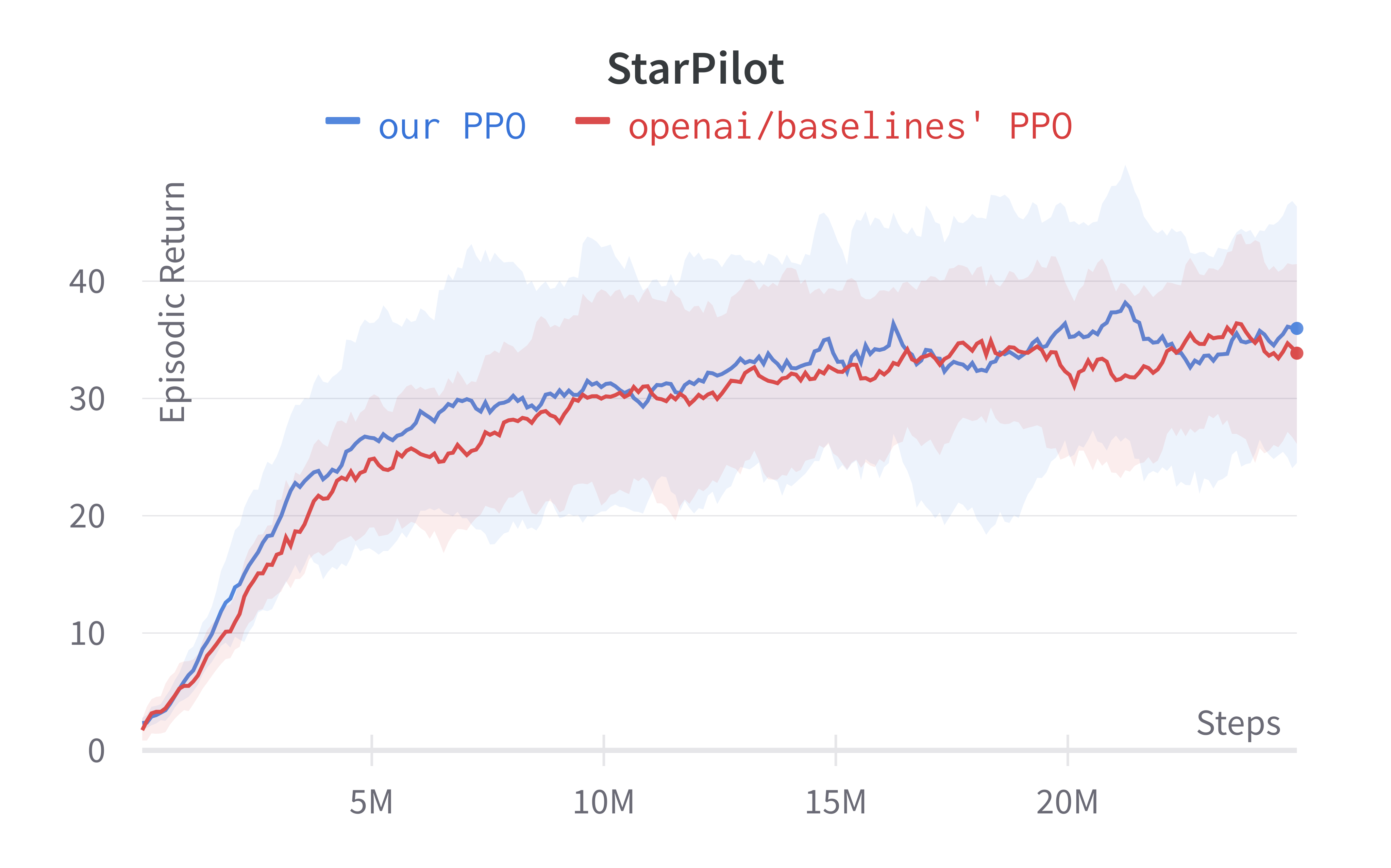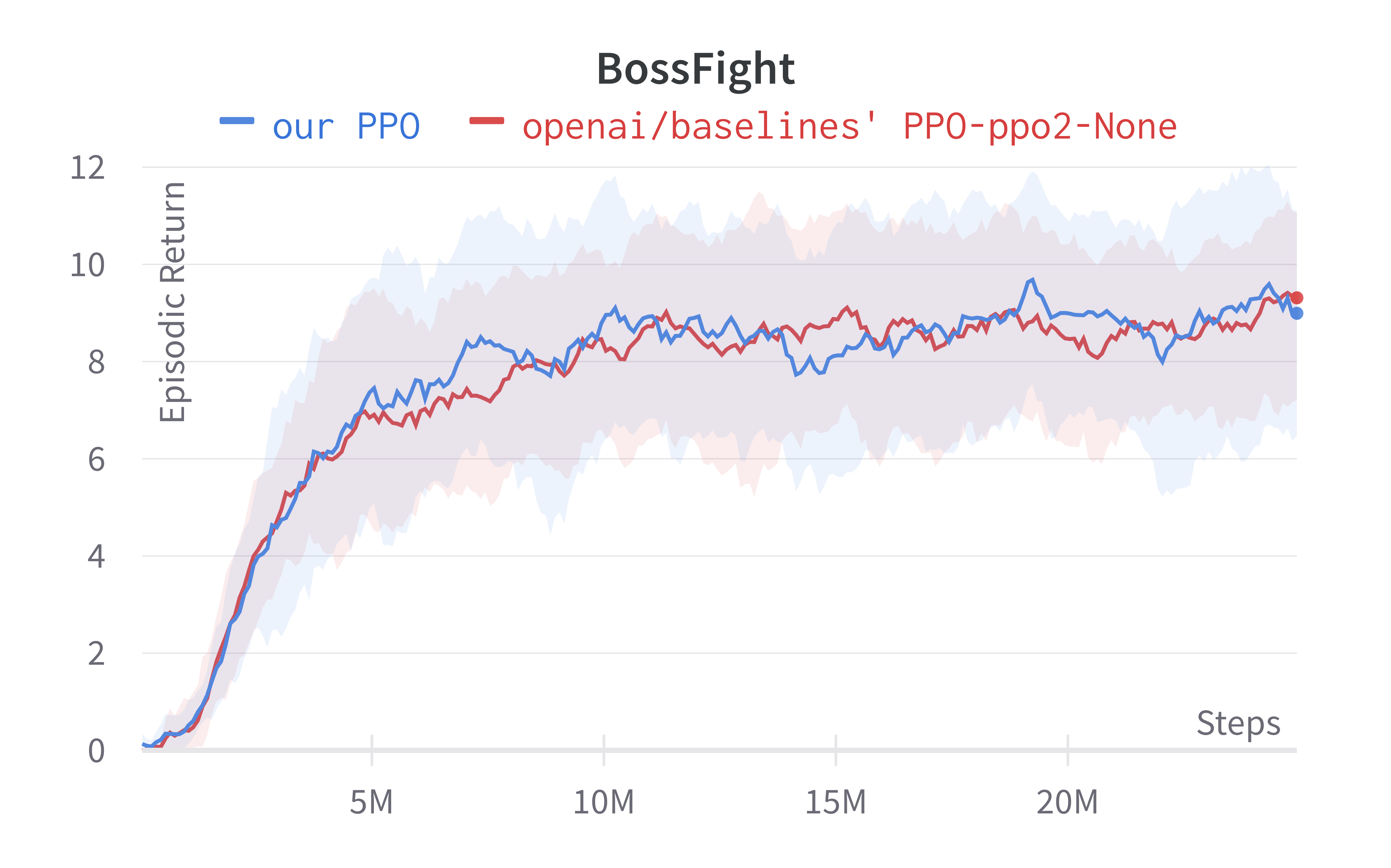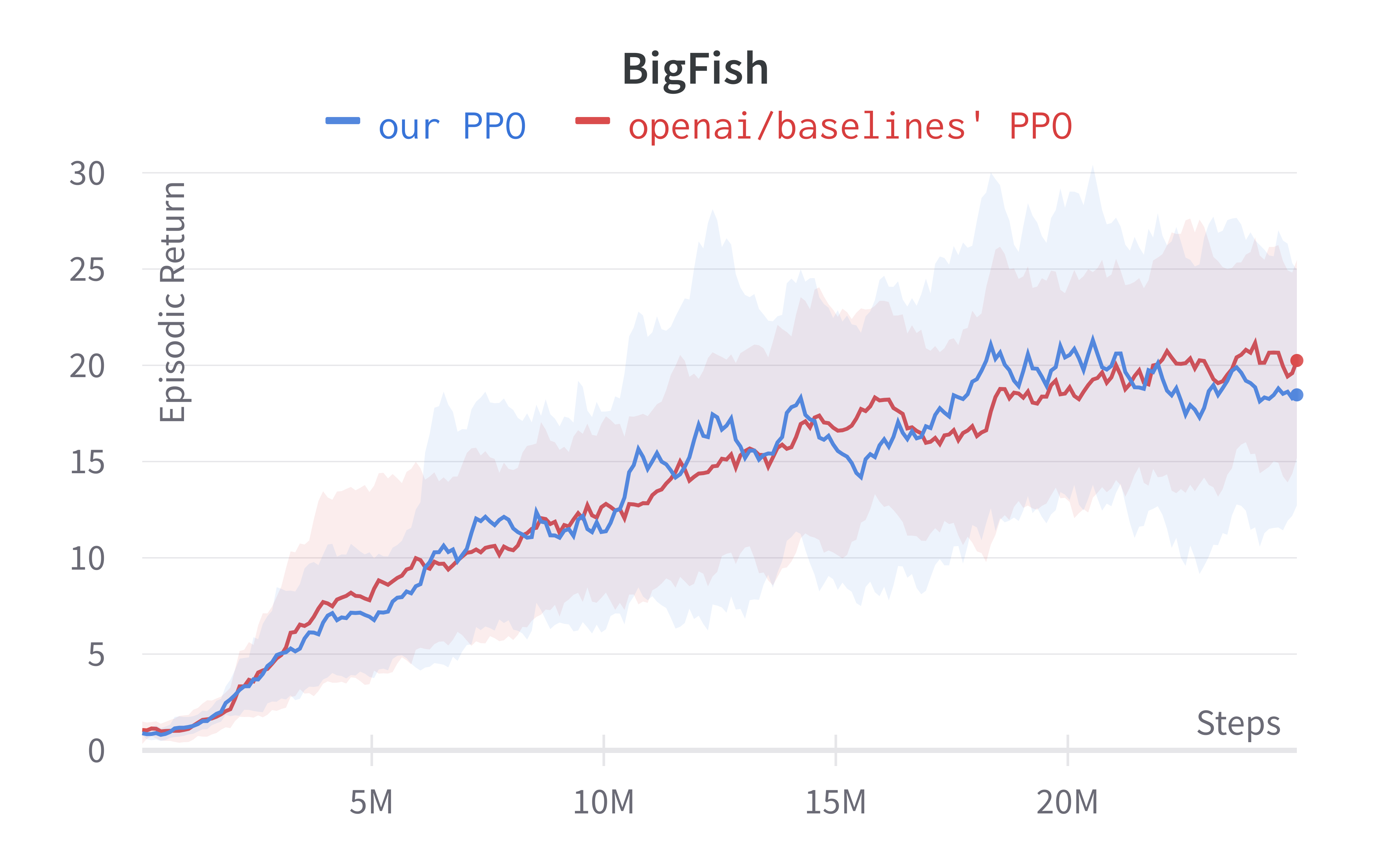
|
||
|
||
> Tracked Procgen experiments (click to show the interactive panel)
|
||
|
||
You will need to sign in to GitHub to add a comment! To edit or delete your comment, visit the [discussions page](https://github.com/iclr-blog-track/iclr-blog-track.github.io/discussions) and look for your comment in the right discussion.
|