PyTorchTS

PyTorchTS is a PyTorch Probabilistic Time Series forecasting framework which provides state of the art PyTorch time series models by utilizing GluonTS as its API (with minimal changes) and for loading, transforming and back-testing time series data sets. Currently the GluonTS code is copied into this repository with changes for PyTorch but eventually GluonTS should become an external requirement.

Installation

$ pip3 install pytorchts

Quick start

Here we highlight the the API changes via the GluonTS README.

import matplotlib.pyplot as plt
import pandas as pd
import torch

from gluonts.dataset.common import ListDataset
from gluonts.dataset.util import to_pandas

from pts.model.deepar import DeepAREstimator
from pts import Trainer

This simple example illustrates how to train a model on some data, and then use it to make predictions. As a first step, we need to collect some data: in this example we will use the volume of tweets mentioning the AMZN ticker symbol.

url = "https://raw.githubusercontent.com/numenta/NAB/master/data/realTweets/Twitter_volume_AMZN.csv"
df = pd.read_csv(url, header=0, index_col=0, parse_dates=True)

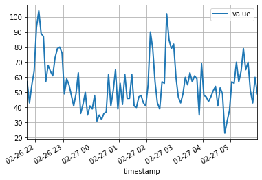
The first 100 data points look like follows:

df[:100].plot(linewidth=2)
plt.grid(which='both')
plt.show()

We can now prepare a training dataset for our model to train on. Datasets are essentially iterable collections of dictionaries: each dictionary represents a time series with possibly associated features. For this example, we only have one entry, specified by the "start" field which is the timestamp of the first data point, and the "target" field containing time series data. For training, we will use data up to midnight on April 5th, 2015.

training_data = ListDataset(
    [{"start": df.index[0], "target": df.value[:"2015-04-05 00:00:00"]}],
    freq = "5min"
)

A forecasting model is a predictor object. One way of obtaining predictors is by training a correspondent estimator. Instantiating an estimator requires specifying the frequency of the time series that it will handle, as well as the number of time steps to predict. In our example we're using 5 minutes data, so req="5min", and we will train a model to predict the next hour, so prediction_length=12. The input to the model will be a vector of size input_size=43 at each time point. We also specify some minimal training options in particular training on a device for epoch=10.

device = torch.device("cuda" if torch.cuda.is_available() else "cpu")

estimator = DeepAREstimator(freq="5min",
                            prediction_length=12,
                            input_size=43,
                            trainer=Trainer(epochs=10,
                                            device=device))
predictor = estimator.train(training_data=training_data, num_workers=4)

    45it [00:01, 37.60it/s, avg_epoch_loss=4.64, epoch=0]
    48it [00:01, 39.56it/s, avg_epoch_loss=4.2, epoch=1] 
    45it [00:01, 38.11it/s, avg_epoch_loss=4.1, epoch=2] 
    43it [00:01, 36.29it/s, avg_epoch_loss=4.05, epoch=3]
    44it [00:01, 35.98it/s, avg_epoch_loss=4.03, epoch=4]
    48it [00:01, 39.48it/s, avg_epoch_loss=4.01, epoch=5]
    48it [00:01, 38.65it/s, avg_epoch_loss=4, epoch=6]   
    46it [00:01, 37.12it/s, avg_epoch_loss=3.99, epoch=7]
    48it [00:01, 38.86it/s, avg_epoch_loss=3.98, epoch=8]
    48it [00:01, 39.49it/s, avg_epoch_loss=3.97, epoch=9]

During training, useful information about the progress will be displayed. To get a full overview of the available options, please refer to the source code of DeepAREstimator (or other estimators) and Trainer.

We're now ready to make predictions: we will forecast the hour following the midnight on April 15th, 2015.

test_data = ListDataset(
    [{"start": df.index[0], "target": df.value[:"2015-04-15 00:00:00"]}],
    freq = "5min"
)

for test_entry, forecast in zip(test_data, predictor.predict(test_data)):
    to_pandas(test_entry)[-60:].plot(linewidth=2)
    forecast.plot(color='g', prediction_intervals=[50.0, 90.0])
plt.grid(which='both')

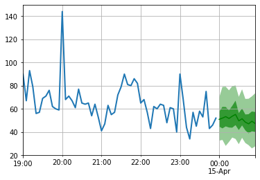
Note that the forecast is displayed in terms of a probability distribution: the shaded areas represent the 50% and 90% prediction intervals, respectively, centered around the median (dark green line).

Development

pip install -e .
pytest test

Scientific Article

We have implemented the following model using this framework:

• Multi-variate Probabilistic Time Series Forecasting via Conditioned Normalizing Flows

@article{rasul2020tempflow,
    Author = {Kashif Rasul, Abdul-Saboor Sheikh, Ingmar Schuster, Urs Bergmann, Roland Vollgraf}
    Title = {Multi-variate Probabilistic Time Series Forecasting via Conditioned Normalizing Flows},
    Year = {2020},
    archivePrefix = {arXiv},
    eprint = {2002.06103},
}

• Autoregressive Denoising Diffusion Models for Multivariate Probabilistic Time Series Forecasting

@article{rasul2020timegrad,
    Author = {Kashif Rasul, Calvin Seward, Ingmar Schuster, Roland Vollgraf}
    Title = {Autoregressive Denoising Diffusion Models for Multivariate Probabilistic Time Series Forecasting},
    Year = {2021},
    archivePrefix = {arXiv},
    eprint = {2101.12072},
}